This is the blog section. It has two categories: News and Releases.
Files in these directories will be listed in reverse chronological order.
This the multi-page printable view of this section. Click here to print.
This is the blog section. It has two categories: News and Releases.
Files in these directories will be listed in reverse chronological order.
SudoSimGUI supports Windows, Linux, and MacOS, with two versions: Server and Client. Users can run the server-side command-line program on a remote server and use the local client for remote connection and real-time visualization and debugging.
Execute in the command line,
sudosim -n -s hostname -p port
where ‘-n’ means not using GUI to run the server program; ‘hostname’ is the server address, default is localhost; ‘port’ is the server port, default is 9091.
SudoDEM is developed based on the Linux platform and provides binary installation (compressed) packages for Ubuntu distributions (14.04-18.04). Simply extract and use without root permissions, no writing to system core directories, completely “green”. In the later stages of the project, Singularity container binary packages will be provided for any Linux distribution.
if you are a programming beginner or Linux beginner:
  it is recommended to try the compiled binary package first
  please continue reading this article
else:
  you can directly download the source code for compilation
  you can quickly skip this article
If you can easily understand the meaning expressed in the code block above, then you can continue reading, otherwise, please directly scroll to the end of the article and like it.
To use SudoDEM, you only need to master the most basic Linux system knowledge and Python programming skills. This article will introduce these essential knowledge. First, please prepare a Linux system, Ubuntu 14-18 is recommended; you can get a Linux system through the following options:
Taking Ubuntu system as an example (commands may vary slightly for different Linux distributions such as CentOS), here are the most basic commands and shortcuts:
The path/directory can be a relative path or absolute path.
Among them, the absolute path starts from the Linux root directory (/), such as: /bin, /home/sway, etc. To facilitate access to user directories (such as /home/sway/), the system gives an abbreviated directory for user directories, represented as ~; ~ is equivalent to the aforementioned /home/sway. Note that Linux system is naturally multi-user, allowing multiple users to log in to the same system at the same time (but each has their own running environment, these configurations are saved in their respective user directories; note: “simultaneous login” does not mean accessing the same desktop). For example, user sway has logged into the system for work, user SC can enter the system through the network (such as ssh remote login command) to work; different users do not interfere with each other (except for competing for hardware resources, such as everyone using SudoDEM for calculations). Relative paths are based on a specific directory. Strictly speaking, paths based on the root directory can also be called relative paths. Because there is never absolute (). In addition to the root directory marker (/) and user directory marker (~), there are two specific symbols used for relative paths (one dot . and two dots ..). One dot (.) represents the current working path, which is the path seen after executing pwd; two dots (..) represent the parent directory relative to the current path. For example, cd ../sub means switching the path to the subdirectory under the parent directory; cd ../../ means switching to the parent directory of the parent directory; cd ./sub switches to the subdirectory under the current directory, of course you can directly type cd sub. Run executable file (program) prog: prog or ./path/prog. If prog can be recognized by the terminal, that is, prog has been added to the system search path (generally the PATH environment variable), you only need to type the executable file name (such as the aforementioned cd is a system command, already in the system default search path). Otherwise, you need to add the path of prog (here ./ means executing this file).
Force terminate terminal program: CTRL+C
$> sudo apt−get install python−numpy
$> pwd
$> cd /home/
$> sudodem3d
Python and C++ mixed programming is the current mainstream trend in computational software. Among them, Python mainly plays the role of interface calling, achieving rapid modeling; while the heavy core computing part is implemented by underlying C++ computing modules. SudoDEM currently still uses Python 2.7 version, and subsequent project development and upgrades will use Python 3.0+ version. It should be pointed out that Python 3 is a comprehensive upgrade of Python 2 and is not backward compatible, but in SudoDEM, we only need the most basic functions (basic syntax is still consistent). The following Python script shows the most basic introductory knowledge.
|
|
Download the latest binary installation package from the SudoDEM project website (https://sudodem.github.io) Download page. Or directly go to SudoDEM’s Github repository (https://github.com/SudoDEM/SudoDEM/releases) to download the compiled binary package.
Extract the binary package to a local directory (such as user directory /home/xxx/), and you will get the following file directory (taking SudoDEM3D as an example):
Through the user configuration file .bashrc (/home/xxx/.bashrc), add the path of the executable file sudodem3d (/home/xxx/SudoDEM/bin) to the environment variable PATH:
PATH=${PATH}:/home/xxx/SudoDEM/bin
Here is a video that may guide you to compile SudoDEM. You can copy the command lines directly from this video.
Non-root permission compilation and installation is the recommended installation method for SudoDEM. Significantly different from Windows, installing software to the system under Linux will install various parts of the software to corresponding directories of the system. For example, compiled binaries will be installed to the bin directory (such as /bin), dynamic link libraries (in order to compile independent functional modules into separate binary library files for development and other reasons, the main program dynamically calls these library files as needed) will be installed to lib (such as /lib), etc. Installation is simple, but uninstallation may have problems. Installing software to the system with sudo permissions (generally through sudo apt install package) often attaches installation of some dependency libraries (skip if already exists); when uninstalling software, if you choose to uninstall dependency libraries at the same time, it may cause other software to not work properly (the required dependency libraries are uninstalled). Choosing non-root permission installation can have many benefits: avoid the above uninstallation problems, can compile and use specific versions of dependency libraries (not using the system’s), and the system is more lightweight. The latest SudoDEM code provides a one-click compilation installation script (shell script), which can be executed directly in the terminal to automatically download the source code of third-party dependency libraries for compilation and installation. First, download the source code from the SudoDEM code repository, and the file structure is as follows:
Among them, the file INSTALL provides detailed installation instructions, including one-click compilation installation and distributed manual compilation installation. Then, create the third-party dependency library compilation directory 3rdlib, SudoDEM2D and SudoDEM3D compilation directories build2d and build3d (as needed), and the local installation directory of SudoDEM sudodeminstall. The final file directory structure is as follows:
Compilation and installation operations are performed in the scripts directory, which contains the installation scripts as follows:
The first step, install third-party libraries:
./install3rdlibs.sh
If the current system does not have the necessary compilation tools installed, this script will automatically install them and require entering the administrator password. Third-party libraries include Boost, Eigen, libQGLViewer, and Minieigen, shared by both SudoDEM2D and 3D, only need to be compiled and installed once. The second step, install the SudoDEM program (taking SudoDEM3D as an example):
./firstCompile_SudoDEM3D.sh
Note: This script is only used for the first compilation and installation; if you have changed the SudoDEM code, you only need to execute make install in the compilation directory (build2d or build3d) to recompile and install. If you have added cpp files in the SudoDEM source code file directory, you need to re-cmake (i.e., cmake ../SudoDEM3D).
Compared with spherical particles, the Newton-Euler equations for non-spherical particle motion adopt a more general form, as follows: \begin{equation}\label{eqnewton_nonsph} m\frac{dv_i}{dt} = F_i \end{equation} where $i\in {1,2,3}$ represents the global Cartesian coordinate axes; $m$ is the particle mass; $v_i$ is the particle translational velocity, the dot above represents differentiation with respect to time, the same below; $F_i$ is the resultant external force acting on the particle center of mass. \begin{equation}\label{eqeuler_nonsph} I_{i}\dot{\omega}_i - (I_{j} - I_{k})\omega_{j} \omega_{k}=M_{i} \end{equation} where $i \in {1,2,3}$ represents the principal axis of inertia, $i$, $j$, $k$ are cyclic indices; $I_i$ is the principal moment of inertia; $\omega_i$ is the angular velocity; $M_i$ is the resultant moment about the particle center of mass. The forces acting on the particle include body forces and contact forces. Compared with the contact forces between spherical particles, a significant feature of the contact forces between non-spherical particles is that the normal component of the contact force (normal contact force) usually does not pass through the particle center of mass, thus can generate a moment about the center of mass. This moment can promote or inhibit the rotation of non-spherical particles. Compared with the simplified Euler equation for spherical particles, the rotational equation of non-spherical particles in equation \eqref{eqeuler_nonsph} involves the asymmetry of principal moments of inertia. The Newton and Euler equations describing particle motion can be solved separately by standard and extended leapfrog algorithms. In addition, for numerical processing convenience, local Cartesian coordinate axes are aligned with the principal axis directions of the particle moment of inertia at the initial moment.
Furthermore, compared with the spherical particle discrete element model, the contact detection in the non-spherical particle discrete element model is much more complex, which is also an important difference between the two. Existing studies have shown that in the process of numerical simulation using the discrete element method, the vast majority of computational resources are consumed in the calculation of contact detection between particles. For non-spherical particle discrete element simulation, this is even more so, and is more time-consuming than spherical particle discrete element simulation. Despite this, given the importance of particle shape, conducting non-spherical particle discrete element research is of great significance. Methods for modeling non-spherical particles are mainly divided into two categories: one is based on spherical discrete elements, using sphere bundling technology to approximate target-shaped particles, i.e., clump discrete element model; the other is based on particle models with precise geometric descriptions, such as polyhedral particles, super-ellipsoidal particles, etc. The content arrangement of this chapter is as follows: first, a brief introduction to the clump discrete element model; then, polyhedral discrete element model and super-ellipsoidal discrete element model are proposed, these two models are used for discrete element modeling of angular and smooth particles respectively in subsequent studies of this paper; finally, the numerical solution of non-spherical particle motion is introduced, and the non-spherical particle discrete element program SudoDEM is independently developed.
Clump particles are non-spherical particles constructed by bundling a series of spheres (hereinafter referred to as component spheres), mainly divided into two types (see Figure 1.1: one is where component spheres can have overlaps, also known as clump model; the other is where there is no overlap between component spheres, also known as cluster model. Note, the overlap here represents much larger than the normal contact overlap in DEM. The classification of the above two clump models is mainly based on the following practical purposes: the clump model can be purely used to represent non-spherical particles, without involving the calculation of contact forces between internal component spheres; the cluster model involves the calculation of contact forces between component spheres, i.e., internal particle forces can be solved, and this model is often used for simulations considering particle breakage.
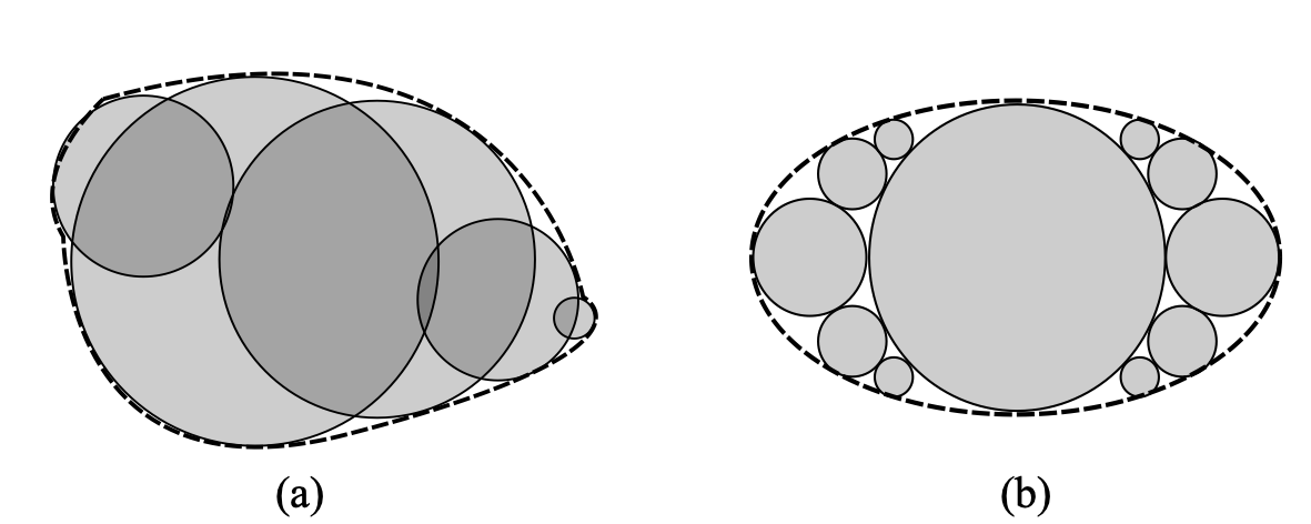
Two-dimensional schematic of two types of clump models: (a) clump model; (b) cluster model
From the definition of clump particles, the degree of approximation to the target non-spherical particle shape is directly related to the number of component spheres. Generally, the more component spheres, the better the clump particles can approximate the target particle. In addition, the arrangement of component spheres in clump particles can be arbitrary, so the clump model has great flexibility. Theoretically, clump particle models can be used to construct particles of any complex shape. However, in practice, a large number of component spheres will significantly increase simulation computation time. In view of this, some scholars [@ashmawy2003] have conducted related research on the construction of non-spherical particle clump models, trying to use as few component spheres as possible to construct particles.
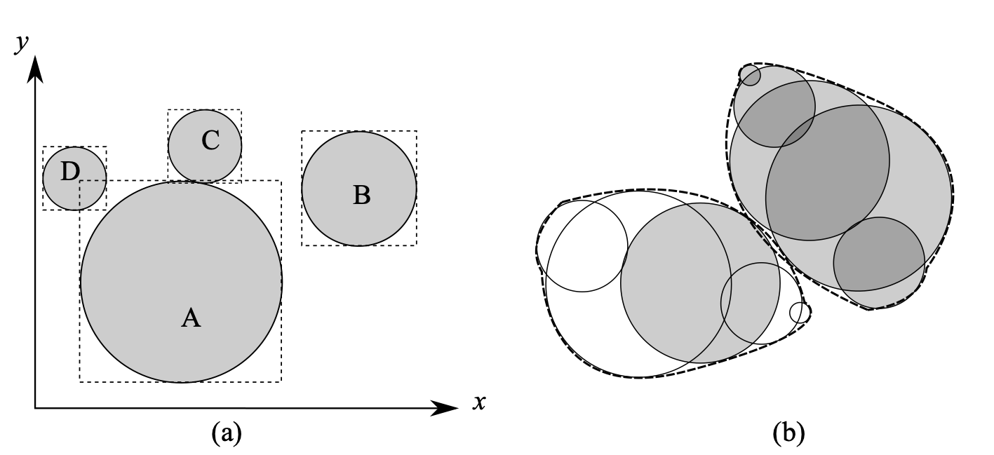
The contact detection of clump particles is based on the contact detection of component spheres, that is, the particle contact detection is achieved by detecting the contact of component spheres of two particles, thus greatly reducing the complexity of contact detection between non-spherical particles. The contact detection between component spheres (as shown in Figure 1.2{reference-type=“ref” reference=“figclumpcontact”}(b)) is completely the same as the contact detection in the spherical discrete element model (as shown in Figure 1.2{reference-type=“ref” reference=“figclumpcontact”}(a)). However, it should be pointed out that to accelerate contact detection, component spheres belonging to the same particle can be exempted from contact detection (only for clump models). The distance between two spherical particles has contact only when the following conditions are met: \begin{equation}\label{eqspherecontact} d_{ij} < R_i + R_j \end{equation} where $d_{ij}$ is the distance between the centers of mass of two spherical particles; $R_i$ and $R_j$ are the radii of the two particles respectively. For two mutually contacting spherical particles, the contact overlap (generally contact penetration depth) $\delta$ is: \begin{equation}\label{eqspheredelta} \delta = R_i + R_j - d_{ij} \end{equation} Other contact geometric quantities can also be easily obtained, such as the contact normal is defined as the direction of the line connecting the centers of mass of the two particles, which is omitted here. It is worth emphasizing that here and in subsequent chapters of this paper, only contacts between non-cohesive particles are involved; for contacts between cohesive particles, equation ([\eqspherecontact]](#eqspherecontact){reference-type=“ref” reference=“eqspherecontact”}) needs to consider that there may be a certain gap between particles, so $\delta$ in equation ([\eqspheredelta]](#eqspheredelta){reference-type=“ref” reference=“eqspheredelta”}) can take negative values, i.e., simulating the cohesive force after particle separation.
 {#figclumpcontact
width=“12cm”}
{#figclumpcontact
width=“12cm”}
It should be noted that in each DEM calculation cycle, a large number of contact detections between particles need to be performed, and each particle only contacts with a few (relative to the large number of particles in the system) surrounding particles, that is, a given particle has no contact with the vast majority of particles. Therefore, to avoid using equation ([\eqspherecontact]](#eqspherecontact){reference-type=“ref” reference=“eqspherecontact”}) for precise contact detection judgment for these large numbers of non-contacting particle pairs, it is usually necessary to first use a sweep and prune algorithm [@baraff1992] to exclude these large numbers of non-contacting particle pairs. Bounding box algorithms are a class of effective screening methods, widely used bounding boxes include spherical bounding boxes, axis-aligned bounding boxes, and oriented bounding boxes. Among them, the axis-aligned bounding box (AABB) [@bergen1997] algorithm is the most popular in DEM particle contact detection. As the name suggests, AABB is a cubic box surrounding the object with six faces aligned with the global coordinate axes, and in most cases, AABB can relatively compactly surround the particle. As shown in Figure 1.2{reference-type=“ref” reference=“figclumpcontact”}(a), the rectangular box is the axis-aligned bounding box. By comparing the length of the projection on each axis, the overlap between two AABBs can be detected. If there is an axis where the AABB projections do not overlap (as shown in Figure 1.2{reference-type=“ref” reference=“figclumpcontact”}(a) where the projections of particle A and particle B’s bounding boxes on the x-axis do not overlap), then there is no overlap between the two AABBs, which also means that the two particles do not overlap. If there is overlap between two AABBs (as shown in Figure 1.2{reference-type=“ref” reference=“figclumpcontact”}(a) where particle A and particle C, particle D have overlapping AABBs), then there may be overlap between the two particles (as shown in Figure 1.2{reference-type=“ref” reference=“figclumpcontact”}(a) where particle A contacts particle C while particle A does not contact particle D). The axis-aligned bounding box algorithm can exclude all particle pairs similar to particles A and B.
As mentioned earlier, the contact between clump particles is essentially the contact between component spheres from different particles. Therefore, traditional spherical discrete element contact models can be directly used for clump discrete element models. Taking the contact stiffness model as an example, we can flexibly choose linear stiffness models, volumetric stiffness models, and other nonlinear stiffness models (such as simplified Hertz-Mindlin model). The linear stiffness model and volumetric stiffness model will be specifically introduced in subsequent sections of this chapter, and are omitted here.
In algebraic geometry, we can define an N-faced convex polyhedron as a convex envelope set composed of N enclosing planes ${p_i|i=1,\dots,N}$, i.e., a set of inequalities: \begin{equation}\label{eqpolydef} P={(x,y,z)|a_ix+b_iy+c_iz\leq d_i,\quad{}i=1,\dots,N} \end{equation} where $(a_i,b_i,c_i)$ is the normal vector of the $i$-th enclosing plane $p_i$, and $d_i$ is the distance from $p_i$ to the origin.
The basic geometric parameters of polyhedra (such as surface area, volume, centroid coordinates, moments of inertia, etc.) can be obtained through classical computational geometry algorithms. For example, when solving the volume of a polyhedron, it can be first divided into a series of tetrahedra, and then the volumes of these tetrahedra can be summed. The solution ideas for other geometric parameters are similar, and are omitted here.
Figure 1.3{reference-type=“ref” reference=“figpolydem”} shows two mutually contacting polyhedral particles, where the overlapping part between the particles is exaggeratedly displayed. Contact detection between polyhedral particles has received much attention, especially in the field of computational geometry. Given a pair of potentially contacting polyhedral particles, denoted as $P_A$ and $P_B$, whether the two polyhedra are in contact is equivalent to whether the two convex sets have an intersection.

Contact detection between polyhedral particles is much more complex than between spherical particles. For spherical particles, the overlap between two particles can be quickly obtained based on their positions and radii, see equation ([\eqspherecontact]](#eqspherecontact){reference-type=“ref” reference=“eqspherecontact”}). However, for polyhedral particles, the overlapping region (see Figure 1.3{reference-type=“ref” reference=“figpolydem”}) is irregular, and it has multiple contact points (for example at face-face or face-edge contacts). Therefore, in most cases, calculating the overlap of two polyhedral particles is time-consuming. Since contact detection between a large number of particles needs to be performed at each time step, we can divide the contact detection into two processes (approximate contact detection and precise detection) to reduce computation time.
To accelerate the contact detection process, we first use the axis-aligned bounding box (AABB) algorithm for rough contact detection. For a brief introduction to the AABB algorithm, see the previous section of this chapter. For particle pairs that cannot be excluded by the AABB algorithm, further precise detection needs to be performed to determine whether there is contact between the two particles. In this case, we use the separating axis (or separating plane) algorithm for further contact detection. Imagine that there exists a separating plane $S={(x,y,z) | a_sx + b_sy+ c_sz = d_s }$ such that all vertices from polyhedron $P_\mathrm{A}$ and $P_\mathrm{B}$ are on opposite sides of the separating plane. There are three types of planes that can be candidate separating planes [@elias2014]:
Enclosing planes of polyhedron $P_\mathrm{A}$;
Enclosing planes of polyhedron $P_\mathrm{B}$;
Planes formed by an edge of polyhedron $P_\mathrm{A}$ and an edge of polyhedron $P_\mathrm{B}$ respectively.
If such a separating plane can be found, then there is no contact between the two polyhedral particles, otherwise, the two polyhedral particles are in contact. For two mutually contacting polyhedral particles, it is necessary to further calculate the relevant geometric quantities at the contact, such as contact overlap (penetration depth or volume), contact normal, etc. The related process is described in the next section.
At each contact, corresponding geometric parameters need to be calculated, such as contact overlap, contact center, and contact normal and tangential directions. Among them, the contact overlap can be contact penetration depth or contact overlap volume, and this model adopts contact overlap volume because the specific contact calculation method below can conveniently give the contact overlap volume. It is worth pointing out that the contact between a particle and a wall (plane) is a degenerate form of particle-particle contact, therefore, the focus here is on particle-particle contact calculation.
 {#figshpv
width=“7cm”}
{#figshpv
width=“7cm”}
 {#figpolyint
width=“9cm”}
{#figpolyint
width=“9cm”}
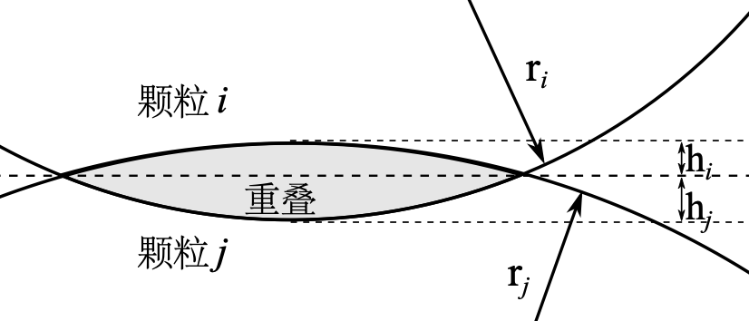
For spherical particles, the contact overlap volume (see Figure 1.4{reference-type=“ref” reference=“figshpv”}) can be obtained through simple geometric calculations, as follows: \begin{equation}\label{eqvsph} v_c=\frac{\pi}{3}[(3r_i-h_i)h_i^2+(3r_j-h_j)h_j^2] \end{equation} where $r_i$(or $r_j$) and $h_i$(or $h_j$) are the radius and spherical cap height of the $i$(or $j$)-th particle respectively. Other geometric parameters can also be given by explicit expressions, which are omitted here.
In contrast, for polyhedral particles, the overlapping region between particles is often an irregular polyhedron, and there is no clear unified theoretical expression to calculate the corresponding geometric parameters. Scholars have successively proposed and developed various precise contact detection algorithms for polyhedral particles, such as the common plane (CP) algorithm [@cundall1988], fast common plane (FCP) algorithm [@nezami2004], and internal potential particle method [@boon2012]. These methods can calculate the penetration depth of polyhedral contacts, but the specific algorithm implementation is relatively cumbersome. Therefore, we use a method based on the so-called duality theory [@muller1978; @gunther1991] to solve the overlapping polyhedron. Interested readers can find more details about this method in the literature [@elias2014; @muller1978; @gunther1991], here only the main operation steps are given, as follows:
Global coordinate system to local coordinate system conversion. The origin of the local coordinate system (hereinafter referred to as the new origin) needs to be set inside the contact overlapping polyhedron. For a new contact, since there is no relevant information in the previous time step, it is necessary to traverse all edges and faces of the two contacting polyhedra until finding a point belonging to the overlap; by moving this point a small distance into the contact overlap, the new origin can be obtained. For an existing contact, the contact point from the previous time step can be used as the new origin.
Mapping from model space to dual space. Model space refers to the space where polyhedra are defined by equation ([\eqpolydef]](#eqpolydef){reference-type=“ref” reference=“eqpolydef”}). In model space, each enclosing plane $p$ from the two polyhedra maps to a point $p^{'}$ in dual space. This mapping relationship is as follows: $$p \Rightarrow p^{'}=(\frac{a}{d},\frac{b}{d},\frac{c}{d})$$ where $a$, $b$, $c$ and $d$ are the plane equation parameters of the enclosing plane $p$.
Solve the convex hull of all $p^{'}$ in dual space. Given that the new origin is inside the contact overlap, $p^{'}$ always exists. In model space, the farther the enclosing plane is from the new origin, the closer the corresponding point in dual space will be to the new origin. Therefore, the convex hull of all dual points corresponds to the contact overlap.
Map the convex hull obtained from the previous step back to model space according to the following mapping relationship: $$q^{'} \Rightarrow q=(\frac{a^{'}}{d^{'}},\frac{b^{'}}{d^{'}},\frac{c^{'}}{d^{'}})$$ where $q^{'}$ is the convex hull enclosing plane in dual space; $a^{'}$, $b^{'}$, $c^{'}$ and $d^{'}$ are the plane equation parameters of $q^{'}$; $q$ is a point of the contact overlap in model space. The convex hull of all contact overlap points $q$ in model space is the contact overlap polyhedron to be solved.
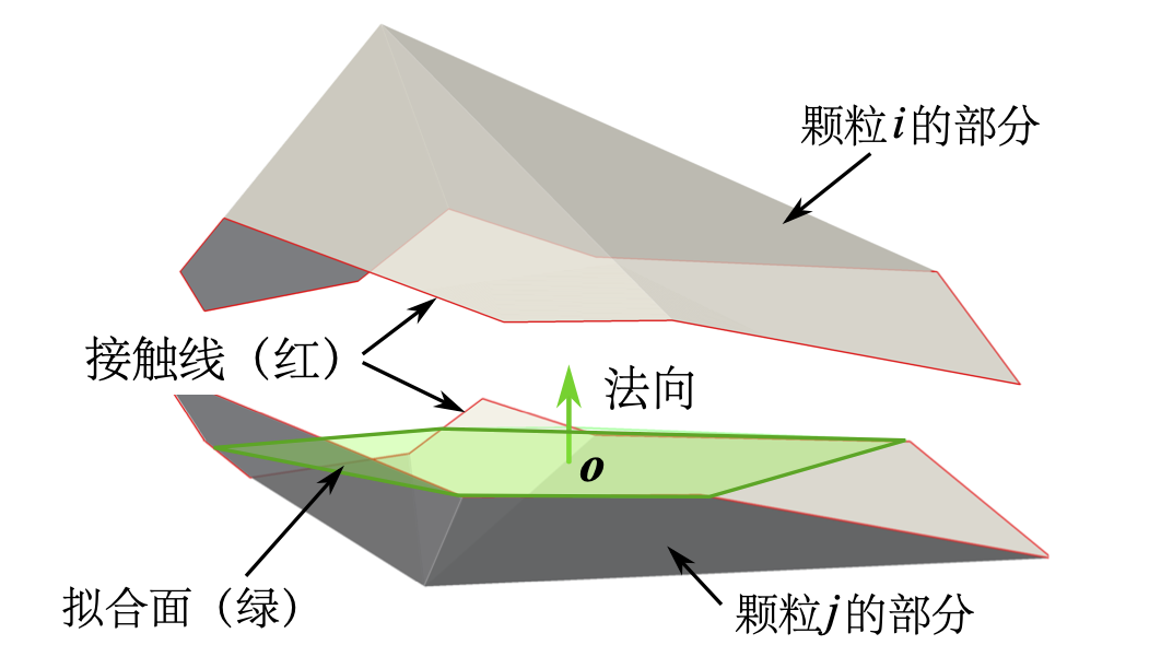
According to the obtained contact overlap polyhedron, the contact direction and contact point can be easily solved through classical computational geometry algorithms. Here, we introduce the contact intersection line to determine the contact normal. The contact intersection line is the intersection line of the surfaces of the two contacting particles, see Figure 1.3{reference-type=“ref” reference=“figpolydem”} or Figure 1.5{reference-type=“ref” reference=“figpolyint”}. Figure 1.5{reference-type=“ref” reference=“figpolyint”} shows the intersecting polyhedron of the two contacting polyhedra (see Figure 1.3{reference-type=“ref” reference=“figpolydem”}). For all component line segments of the contact intersection line, a fitting plane is fitted using the least squares method, and the normal of this fitting plane is assumed to be the contact normal, and the direction orthogonal to this normal is the tangential direction. It is worth noting that the tangential direction here is strictly the plane where the tangential direction lies (tangent plane), and the specific contact tangential is related to the relative displacement of the two particles in this tangent plane. For spherical particles, the contact intersection line is strictly located on the fitting plane, see Figure 1.4{reference-type=“ref” reference=“figshpv”}, but this is not the case for polyhedral particles. In addition, the centroid of the overlapping part (polyhedron) can be assumed as the contact point, i.e., the point where the contact force acts. It is worth pointing out that the above definitions of contact normal and contact point are very approximate, because the overlapping part of the two polyhedra (see Figure 1.3{reference-type=“ref” reference=“figpolydem”}) is irregular, and there are actually multiple contact points, for example at face-face or face-edge contacts. In addition, in most cases, the contact point does not lie on the fitting plane.
The contact stiffness model, as a commonly used contact model in DEM, defines the elastic relationship between contact force $F$ and relative displacement $\delta$, see equation ([\eqlaw]](#eqlaw){reference-type=“ref” reference=“eqlaw”}). For ease of description and modeling, the contact force is usually divided into two orthogonal components: the tangential contact force $F_t$ on the contact plane and the normal contact force $F_n$ in the normal direction of the contact plane, as shown in Figure 1.3{reference-type=“ref” reference=“figpolydem”}. It should be noted that the contact plane is considered to be obtained by least squares fitting of the intersection curve of the two polyhedra [@elias2014]. \begin{equation}\label{eqlaw} F=K\delta \end{equation} where $K$ is the contact stiffness, determined by the material properties of the contacting particles. If the contact stiffness $K$ is constant throughout the computational simulation process, then equation ([\eqlaw]](#eqlaw){reference-type=“ref” reference=“eqlaw”}) defines a linear elastic contact model. The contact stiffness $K$ in this paper is given by equation ([\eqK]](#eqK){reference-type=“ref” reference=“eqK”}), where the superscripts A and B represent the two contacting particles. \begin{equation}\label{eqK} K=\frac{K^AK^B}{K^A+K^B} \end{equation}
Usually, the contact overlap $\delta$ in equation ([\eqlaw]](#eqlaw){reference-type=“ref” reference=“eqlaw”}) is the penetration depth. Here, a normal contact model applicable to arbitrary particle shapes is adopted. As shown in equation ([\eqvlaw]](#eqvlaw){reference-type=“ref” reference=“eqvlaw”}), the normal contact force is related to the contact overlap volume. This normal contact model has been used by other scholars [@chen2010; @nassauer2013; @nassauer2013c; @elias2014]. \begin{equation}\label{eqvlaw} F\_n=K\_nv\_c \end{equation} where $K_n$ [N/m$^3$] is the contact normal stiffness (volumetric stiffness), given by equation ([\eqK]](#eqK){reference-type=“ref” reference=“eqK”}); $v_c$ [m$^3$] is the contact overlap volume, its detailed calculation is described in the previous section.
In addition, the most commonly used tangential contact model is adopted, as follows: \begin{equation}\label{eqFs} \Delta F\_t=-K\_t \Delta u \end{equation} where $K_t$ [N/m] is the contact tangential stiffness; $\Delta u$ and $\Delta F_t$ are the tangential contact displacement increment and tangential contact force increment at the current time step respectively.
The Coulomb condition or sliding friction model is used to determine contact sliding. When $F_t$ is greater than $\tan\phi_\mu\cdot F_n$ (where $\phi_\mu$ is the sliding friction angle), sliding occurs, and $F_t$ must be reduced and maintained at $\tan\phi_\mu\cdot F_n$. It should be noted that given the relatively small influence of rolling friction [@mack2011], this model does not involve rolling friction.
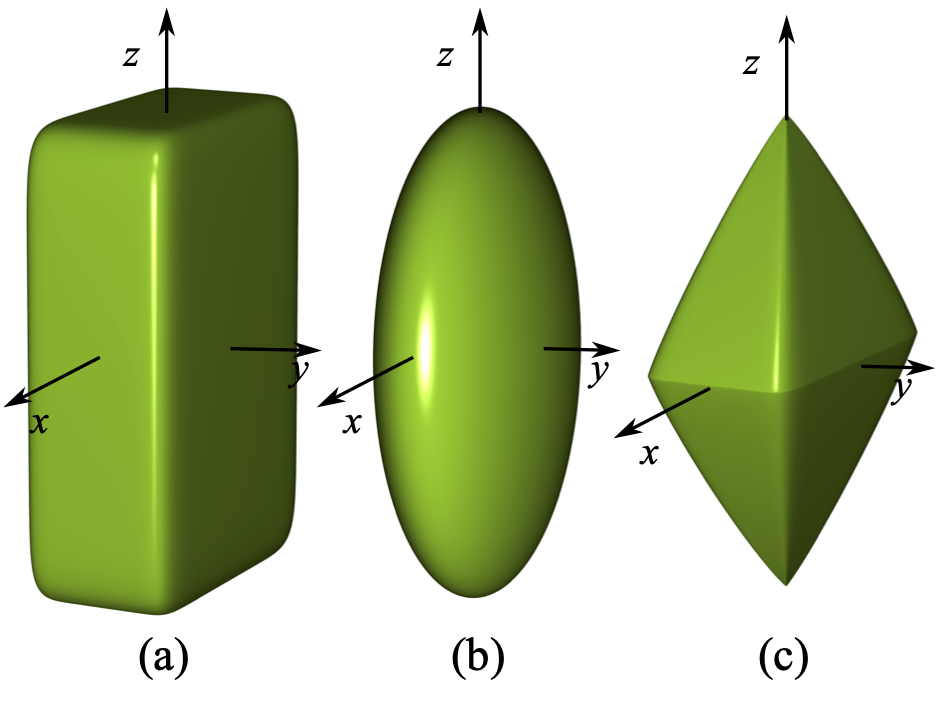
Super-ellipsoid surfaces are a special class of closed super-quadric surfaces that can express rich geometric shapes. In a local Cartesian coordinate system, the surface equation of a super-ellipsoid can be defined as [@barr1981]: \begin{equation}\label{eqsurface_super} (|\frac{x}{a}|^{\frac{2}{\epsilon\_1}} + |\frac{y}{b}|^{\frac{2}{\epsilon\_1}})^{\frac{\epsilon\_1}{\epsilon\_2}} + |\frac{z}{c}|^{\frac{2}{\epsilon\_2}} = 1 \end{equation} where $a$, $b$ and $c$ are the semi-axis lengths in the x, y and z directions respectively, and $\epsilon_i (i=1,2)$ are shape parameters that determine the sharpness of the particle edges. Interested readers can find other similar definitions of super-ellipsoids in the literature [@williams1992; @cleary1997efficient]. This paper mainly studies convex shapes, whose corresponding $\epsilon_i$ are between $(0,2)$. As shown in Figure 1.6{reference-type=“ref” reference=“figsuperellipsoids”}, changing $\epsilon_i$ can obtain various shapes. In particular, $\epsilon_i \rightarrow 0$ corresponds to cubic shapes, while $\epsilon_i \rightarrow 2$ corresponds to octahedral shapes.
 {#figsuperellipsoids
width=“8cm”}
{#figsuperellipsoids
width=“8cm”}
The following gives a series of important geometric parameters of super-ellipsoids involved in this model, such as volume, principal moments of inertia, etc. The volume of a super-ellipsoid is given by: \begin{equation}\label{eqVolume} V = 2AB(\frac{1}{2}\epsilon\_1+1, \epsilon\_1)B(\frac{1}{2}\epsilon\_2, \frac{1}{2}\epsilon\_2)\end{equation} where $A$ equals $abc\epsilon_1\epsilon_2$; $B(x, y)$ is the beta function, defined as $$B(x, y) = 2\int\_0^{\frac{\pi}{2}}\mathrm{sin}^{2x-1}\phi \mathrm{cos}^{2y-1}\phi d\phi = \frac{\Gamma(x)\Gamma(y)}{\Gamma(x+y)}$$ where $\Gamma(x)$ is the gamma function. The principal moments of inertia of the super-ellipsoid are: \begin{equation}\label{eqinertia} \begin{aligned} I\1 &= I\{xx} =\frac{1}{2} \rho A(b^2\beta\_1 + 4c^2\beta\_2) \\ I\2 &= I\{yy} = \frac{1}{2} \rho A(a^2\beta\_1 + 4c^2\beta\_2) \\ I\3 &= I\{zz} = \frac{1}{2} \rho A(a^2 + b^2)\beta\_1 \end{aligned} \end{equation} where $\rho$ is the material density, and parameters $\beta_1$ and $\beta_2$ are defined as follows: \begin{equation}\left{ \begin{array}{l@{}l} \beta\_1 = B(\frac{3}{2}\epsilon\_2, \frac{1}{2}\epsilon\_2)B(\frac{1}{2}\epsilon\_1, 2\epsilon\_1 + 1)\\ \beta\_2 = B(\frac{1}{2}\epsilon\_2, \frac{1}{2}\epsilon\_2 + 1)B(\frac{3}{2}\epsilon\_1,\epsilon\_1+1) \end{array} \right.\end{equation}
Given the parametric equation of a super-ellipsoid as: \begin{equation} \mathbf{r}(\theta,\phi)= \begin{bmatrix} \mathrm{Sign}(\cos\theta)r\_x|\cos\theta|^{\epsilon\_1}|\cos\phi|^{\epsilon\_2} \\ \mathrm{Sign}(\sin\theta)r\_y|\sin\theta|^{\epsilon\_1}|\cos\phi|^{\epsilon\_2} \\ \mathrm{Sign}(\sin\phi)r\_z|\sin\phi|^{\epsilon\_2} \end{bmatrix} \end{equation} and $\theta \in [0,2\pi),\phi \in [-\frac{\pi}{2},\frac{\pi}{2}]$. Where $r_x$, $r_y$ and $r_z$ are the semi-axis lengths in the principal axis directions in the local coordinate system; $\mathrm{Sign}(x)$ represents the sign function, defined as follows: \begin{equation}\label{eqsign} \mathrm{Sign}(x) = \begin{cases} -1 & \text{if} \quad x < 0, \\ 0 & \text{if} \quad x = 0, \\ 1 & \text{if} \quad x > 0. \end{cases}\end{equation}
Therefore, the first and second derivatives of the parametric equation are: \begin{equation}\mathbf{r}\_{\theta}= \begin{bmatrix} -\mathrm{Sign}(\cos\theta)r\_x\epsilon\_1|\cos\theta|^{\epsilon\_1 -2}|\cos\phi|^{\epsilon\_2}\cos\theta\sin\theta \\ \mathrm{Sign}(\sin\theta)r\_y\epsilon\_1|\sin\theta|^{\epsilon\_1-2}|\cos\phi|^{\epsilon\_2}\cos\theta\sin\theta \\ 0 \end{bmatrix} \end{equation}
\begin{equation} \mathbf{r}\_{\phi}= \begin{bmatrix} -\mathrm{Sign}(\cos\theta)r\_x\epsilon\_2|\cos\theta|^{\epsilon\_1}|\cos\phi|^{\epsilon\_2-2}\cos\phi\sin\phi \\ -\mathrm{Sign}(\sin\theta)r\_y\epsilon\_2|\sin\theta|^{\epsilon\_1}|\cos\phi|^{\epsilon\_2-2}\cos\phi\sin\phi \\ \mathrm{Sign}(\sin\phi)r\_z\epsilon\_2|\sin\phi|^{\epsilon\_2-2}\cos\phi\sin\phi \end{bmatrix} \end{equation}
\begin{equation} \begin{aligned} \mathbf{r}\_{\theta\phi}=\frac{\sin2\theta\sin2\phi}{4} \begin{bmatrix} \mathrm{Sign}(\cos\theta)r\_x\epsilon\_1\epsilon\_2|\cos\theta|^{\epsilon\_1-2}|\cos\phi|^{\epsilon\_2-2} \\ -\mathrm{Sign}(\sin\theta)r\_y\epsilon\_1\epsilon\_2|\sin\theta|^{\epsilon\_1-2}|\cos\phi|^{\epsilon\_2-2} \\ 0 \end{bmatrix} \end{aligned} \end{equation}
\begin{equation} \mathbf{r}\_{\theta\theta}= \begin{bmatrix} \mathrm{Sign}(\cos\theta)r\_x\epsilon\_1|\cos\theta|^{\epsilon\_1-2}|\cos\phi|^{\epsilon\_2}(\epsilon\_1\sin^2\theta-1) \\ \mathrm{Sign}(\sin\theta)r\_y\epsilon\_1|\sin\theta|^{\epsilon\_1-2}|\cos\phi|^{\epsilon\_2}(\epsilon\_1\cos^2\theta-1)\\ 0 \end{bmatrix} \end{equation}
\begin{equation} \mathbf{r}\_{\phi\phi}= \begin{bmatrix} \mathrm{Sign}(\cos\theta)r\_x\epsilon\_2|\cos\theta|^{\epsilon\_1}|\cos\phi|^{\epsilon\_2-2}(\epsilon\_2\sin^2\phi-1) \\ \mathrm{Sign}(\sin\theta)r\_y\epsilon\_2|\sin\theta|^{\epsilon\_1}|\cos\phi|^{\epsilon\_2-2}(\epsilon\_2\sin^2\phi-1)\\ \mathrm{Sign}(\sin\phi)r\_z\epsilon\_2|\sin\phi|^{\epsilon\_2-2}(\epsilon\_2\cos^2\phi-1) \end{bmatrix} \end{equation}
The outward normal unit vector on the surface of the super-ellipsoid is:
\begin{equation} \mathbf{n}=\frac{\mathbf{r}\{\theta} \times \mathbf{r}\{\phi}}{| \mathbf{r}\{\theta}\times \mathbf{r}\{\phi} |} \end{equation}
where ‘$\times$’ represents vector cross product, and ‘$|\quad|$’ represents vector magnitude.
First fundamental form coefficients: \begin{equation} E=\mathbf{r}\{\theta}\cdot \mathbf{r}\{\theta} \quad{} F=\mathbf{r}\{\theta}\cdot \mathbf{r}\{\phi} \quad{} G=\mathbf{r}\{\phi}\cdot \mathbf{r}\{\phi} \end{equation}
where ‘$\cdot$’ represents vector dot product. Second fundamental form coefficients: \begin{equation} L=\mathbf{r}\{\theta\theta}\cdot \mathbf{n} \quad M=\mathbf{r}\{\theta\phi}\cdot \mathbf{n}=0 \quad N=\mathbf{r}\_{\phi\phi}\cdot \mathbf{n} \end{equation}
Gaussian curvature: $$K=\frac{LN}{EG-F^2}$$ Mean curvature: $$H=\frac{EN+GL}{2(EG-F^2)}$$ Principal curvatures: \begin{equation}\rho\{I}=H+\sqrt{H^2-K} \quad \rho\{II}=H-\sqrt{H^2-K}\end{equation}
Given a local spherical coordinate $(\theta, \phi)$ of a point on the surface of the super-ellipsoid, the corresponding Cartesian coordinates $(x, y, z)$ can be obtained by the following function $\mathbb{F}_1$: \begin{equation}\label{eqF} \begin{aligned} x =& \mathrm{Sign}(\mathrm{cos}(\theta))a|\mathrm{cos}(\theta)|^{\epsilon\_1} |\mathrm{cos}(\phi)|^{\epsilon\_2}\\ y =& \mathrm{Sign}(\mathrm{sin}(\theta))b|\mathrm{sin}(\theta)|^{\epsilon\_1} |\mathrm{cos}(\phi)|^{\epsilon\_2}\\ z =& \mathrm{Sign}(\mathrm{sin}(\phi))c|\mathrm{sin}(\phi)|^{\epsilon\_2} \end{aligned} \end{equation}
Given a normal vector $(n_x, n_y, n_z)$ on the surface of the super-ellipsoid, the corresponding local spherical coordinates $(\theta, \phi)$ can be obtained by the following function $\mathbb{F}_2$: \begin{equation}\label{eqf} \begin{aligned} \theta = \mathrm{atan2}(\mathrm{Sign}(n\_y)|b n\_y|^{\frac{1}{2 - \epsilon\_1}}, \mathrm{Sign}(n\_x)|an\_x|^{\frac{1}{2 - \epsilon\_1}}) \\ \phi = \mathrm{atan2}(\mathrm{Sign}(n\_z)|cn\_z|\mathrm{cos}(\theta)|^{2 - \epsilon\_2}|^{\frac{1}{2 - \epsilon\_2}}, |an\_x|^{\frac{1}{2 - \epsilon\_2}}) \end{aligned} \end{equation} where $\mathrm{atan2}(x, y)$ is the arctangent function of $\frac{x}{y}$, with value range $(-\pi, \pi]$; $\mathrm{Sign}(x)$ is the sign function, definition see equation ([\eqsign]](#eqsign){reference-type=“ref” reference=“eqsign”}).
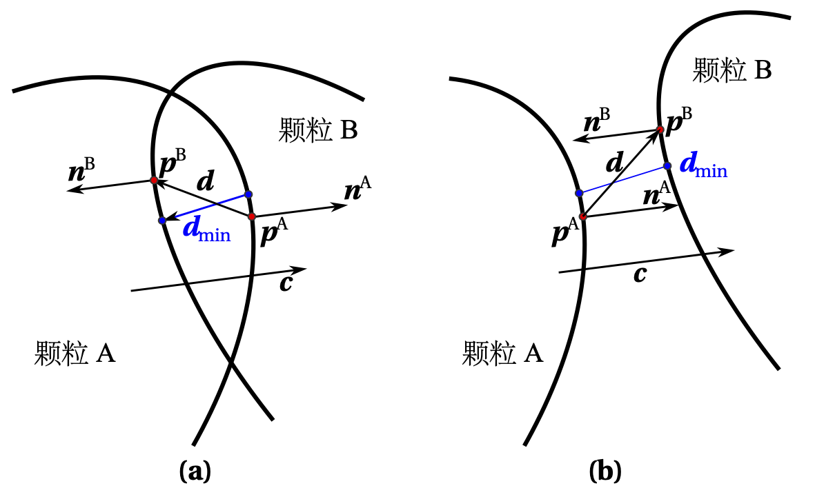
In each loop time step of DEM, the contact penetration depth and direction between particles need to be updated to obtain updated contact forces. Given two potentially contacting adjacent particles A and B, the possible contact points from the two particles are denoted as $\mathbf{p}^A$ and $\mathbf{p}^B$ respectively, and the corresponding potential contact penetration vector is denoted as $\mathbf{d} = (\mathbf{p}^B-\mathbf{p}^A)$, see Figure 1.7{reference-type=“ref” reference=“figdetection”}(a). According to the common normal concept [@johnson1985; @wellmann2008], the contact points to be solved must minimize the contact penetration depth and must simultaneously satisfy the following constraints:
(1) The outward normal unit vectors $\mathbf{n}^A$ and $\mathbf{n}^B$ at the contact points $\mathbf{p}^A$ and $\mathbf{p}^B$ satisfy anti-parallel and are parallel to the contact direction $\mathbf{c}$, i.e.: \begin{equation}\label{eqnnc} \mathbf{n}^A = -\mathbf{n}^B = \mathbf{c}\end{equation}
(2) The potential contact penetration vector $\mathbf{d}$ is parallel to the contact direction $\mathbf{c}$, i.e.: \begin{equation}\label{eqdc} \mathbf{d} \times \mathbf{c} = \mathbf{0}\end{equation} Therefore, finding the target contact point is an optimization problem. As suggested by Wellmann et al. [@wellmann2008], the contact direction $\mathbf{c}$ can be parameterized by two angles in the local spherical coordinate system, i.e.: \begin{equation}\mathbf{c}(\alpha, \beta) = \mathrm{cos}\alpha\mathrm{cos}\beta \mathbf{i}+ \mathrm{sin}\alpha\mathrm{cos}\beta \mathbf{j}+ \mathrm{sin}\beta \mathbf{k}\end{equation} where $\mathbf{i}$, $\mathbf{j}$, $\mathbf{k}$ are the unit basis vectors of the global Cartesian coordinate system. Therefore, considering equation ([\eqnnc]](#eqnnc){reference-type=“ref” reference=“eqnnc”}), the contact points can be expressed as: $$% \left{ \begin{array}{ll} \mathbf{p}^A = \mathbf{T}^{-1}\_A\mathbb{F}\_1^A(\mathbb{F}\_2^A(\mathbf{T}\_A\mathbf{c}(\alpha, \beta))) + \mathbf{s}^A\\ \mathbf{p}^B = \mathbf{T}^{-1}\_B\mathbb{F}\_1^B(\mathbb{F}\_2^B(-\mathbf{T}\_B\mathbf{c}(\alpha, \beta))) + \mathbf{s}^B \end{array} \right.$$ where $\mathbf{T}$ is the rotation matrix from the global coordinate system to the particle’s local coordinate system, $\mathbf{T}^{-1}$ is its inverse matrix; $\mathbf{s}$ is the position vector of the particle in the global coordinate system; $\mathbb{F}_1$ and $\mathbb{F}_2$ are two geometric transformation functions in the particle’s local coordinate system, see equations ([\eqF]](#eqF){reference-type=“ref” reference=“eqF”}) and ([\eqf]](#eqf){reference-type=“ref” reference=“eqf”}). Therefore, finding the penetration depth $||\mathbf{d}||$ is equivalent to solving the following unconstrained optimization problem with two parameters: \begin{equation}\label{eqfinald} \underset{\alpha, \beta}{\mathrm{min}}||\mathbf{d}|| = \underset{\alpha, \beta}{\mathrm{min}}||\mathbf{p}^B - \mathbf{p}^A||\end{equation} This paper adopts the Nelder-Mead simplex algorithm [@lagarias1998] to obtain a robust solution process. It is worth noting that when equation ([\eqfinald]](#eqfinald){reference-type=“ref” reference=“eqfinald”}) reaches the global minimum, equation ([\eqdc]](#eqdc){reference-type=“ref” reference=“eqdc”}) is automatically satisfied [@wellmann2008].
 {#figdetection
width=“10cm”}
{#figdetection
width=“10cm”}
Given that contact detection between a large number of particles needs to be performed at each time step, a combined algorithm of approximate contact detection and precise contact detection can be used to accelerate the contact detection process. First, a two-level approximate contact detection scheme is adopted. In the first level, the axis-aligned bounding box (AABB) algorithm (see Section 2 of this chapter for details) is used to exclude most particle pairs that are not in contact with each other. Given the symmetry of super-ellipsoids, for each particle, a fixed-size cubic AABB is used, i.e., there is no need to recalculate the particle’s AABB at each time step. Then, spherical bounding boxes are used for further screening in the second level. For the remaining potentially contacting particle pairs, precise contact detection is required, see the previous section for details. It should be emphasized that during the optimization solution process, the following condition can be checked at each iteration: \begin{equation}\mathbf{d} \cdot \mathbf{c} > 0\end{equation} If the above condition is satisfied, then there is no contact between the investigated particle pair [@wellmann2008], see Figure 1.7{reference-type=“ref” reference=“figdetection”}(b), therefore, the current particle pair can be excluded and further contact detection for this particle pair can be terminated.
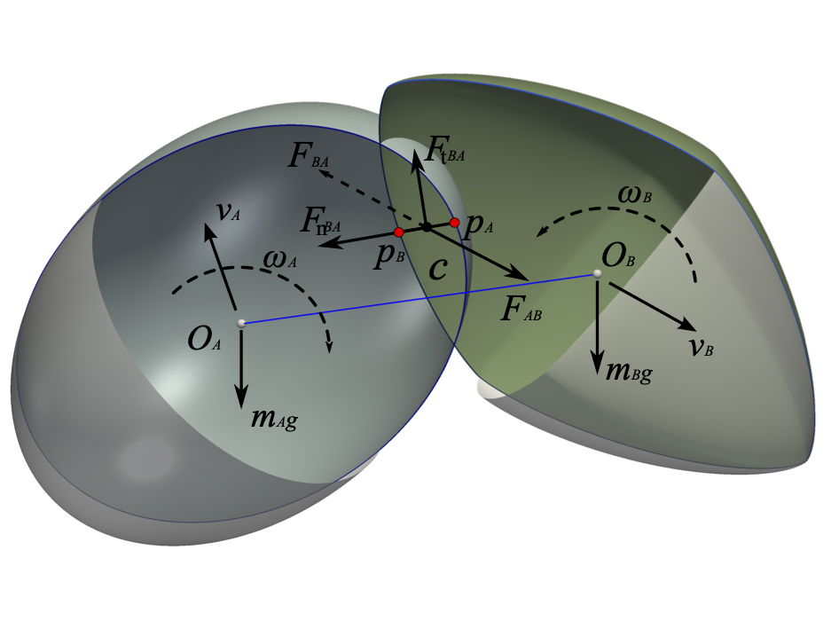
DEM assumes that particles are completely rigid but can overlap between particles (so-called soft sphere model) [@cundall1979], see Figure 1.8{reference-type=“ref” reference=“figsuperedem”}. Therefore, the repulsive force can be calculated according to the given contact constitutive model and current overlap. Currently, scholars have proposed various contact models for different research problems. However, due to the simplicity of the linear spring model [@bagi2003] and its significant improvement in computational efficiency for non-spherical particles (detailed discussion is given in this paper), its use is very widespread. Therefore, most of the numerical simulations in this paper adopt this model, given by: \begin{equation}\left{ \begin{array}{l@{}l} F\_n=\delta K\_n\\ F\_t=\mathrm{min}{F\_t^{'}-\Delta u K\_t, \mu F\n} \end{array} \right.\end{equation} where $F_n$ and $F_t$ are the normal and tangential contact forces respectively; $K_n$ and $K_t$ are the corresponding normal and tangential contact stiffnesses; $\Delta u$ is the contact tangential displacement increment per time step; $\delta$ is the mutual penetration (overlap) depth between particles at the contact; $\mu$ is the friction coefficient between particles; $F_t^{'}$ is the tangential contact force from the previous time step. It should be noted that the Coulomb condition (or sliding friction model) is applied to the calculation of tangential contact force. When contact is formed, the tangential contact force $F_t^{'}$ is initialized to zero. The contact stiffness $K$ ($$ represents $n$ or $t$) is set to the harmonic average of the material stiffnesses of the two contacting particles, see equation ([\equK]](#equK){reference-type=“ref” reference=“equK”}), where the superscripts A and B represent the two contacting particles.
\begin{equation}\label{equK} K\{*}=\frac{2K\{}^AK\_{}^B}{K\{*}^A+K\{*}^B}\end{equation}
 {#figsuperedem
width=“8cm”}
{#figsuperedem
width=“8cm”}
Particle motion can be solved by a time increment $\Delta t$ step-based similar central difference method, i.e., leapfrog strategy, or Verlet strategy [@rapaport2004].
Given the position vector $\mathbf{x}^{t}$ of the particle at the current moment $t$, the linear acceleration $\mathbf{a}^t$ can be calculated by Newton’s equation ([\eqnewton_sph]](#eqnewton_sph){reference-type=“ref” reference=“eqnewton_sph”}), i.e.: \begin{equation}\label{eqtransacc} \mathbf{a}^t = \frac{\mathbf{F}}{m}\end{equation} where $\mathbf{F}$ is the resultant external force including damping force.
Perform Taylor series expansion on the position vectors $\mathbf{x}^{t-\Delta t}$ and $\mathbf{x}^{t+\Delta t}$ of the previous and next time steps respectively: \begin{equation}\mathbf{x}^{t-\Delta t} = \mathbf{x}^{t}-\Delta t \big (\frac{d\mathbf{x}}{dt} \big )^t + \frac{\Delta t^2}{2!} \big (\frac{d^2\mathbf{x}}{dt^2} \big )^t -\frac{\Delta t^3}{3!} \big (\frac{d^3\mathbf{x}}{dt^3} \big )^t +\dots+ (-1)^n\frac{\Delta t^n}{n!} \big (\frac{d^n\mathbf{x}}{dt^n} \big )^t + O(\Delta t^{n+1})\end{equation} \begin{equation}\mathbf{x}^{t+\Delta t} = \mathbf{x}^{t}+\Delta t \big (\frac{d\mathbf{x}}{dt} \big )^t + \frac{\Delta t^2}{2!} \big (\frac{d^2\mathbf{x}}{dt^2} \big )^t +\frac{\Delta t^3}{3!} \big (\frac{d^3\mathbf{x}}{dt^3} \big )^t +\dots+ \frac{\Delta t^n}{n!} \big (\frac{d^n\mathbf{x}}{dt^n} \big )^t + O(\Delta t^{n+1})\end{equation} Therefore, $\mathbf{a}^t$ can also be written in the form of a central difference of the position vector with respect to the time step, i.e.: \begin{equation}\label{eqxtdeltato} \mathbf{a}^t = \frac{\mathbf{x}^{t-\Delta t}-2\mathbf{x}^{t}+\mathbf{x}^{t+\Delta t}}{\Delta t^2} + O(\Delta t^2)\end{equation} Discarding the truncation error and rearranging gives: \begin{equation}\label{eqxtdeltat} \mathbf{x}^{t+\Delta t} = 2\mathbf{x}^{t}-\mathbf{x}^{t-\Delta t}+\mathbf{a}^t\Delta t^2=\mathbf{x}^{t}+\Delta t\big (\frac{\mathbf{x}^{t}-\mathbf{x}^{t-\Delta t}}{\Delta t} + \mathbf{a}^t\Delta t \big )\end{equation} The translational velocity $\mathbf{v}^{t-\frac{\Delta t}{2}}$ at moment $t-\frac{\Delta t}{2}$ can be obtained from the position vectors of the current and previous time steps, i.e.: \begin{equation}\label{eqvt_deltat} \mathbf{v}^{t-\frac{\Delta t}{2}} = \frac{\mathbf{x}^{t}-\mathbf{x}^{t-\Delta t}}{\Delta t}\end{equation} The translational velocity $\mathbf{v}^{t+\frac{\Delta t}{2}}$ at moment $t+\frac{\Delta t}{2}$ can be obtained by the following equation: \begin{equation}\label{eqvtdeltat} \mathbf{v}^{t+\frac{\Delta t}{2}} = \mathbf{v}^{t-\frac{\Delta t}{2}}+\mathbf{a}^t \Delta t\end{equation} Substituting equation ([\eqvt_deltat]](#eqvt_deltat){reference-type=“ref” reference=“eqvt_deltat”}) into equation ([\eqxtdeltat]](#eqxtdeltat){reference-type=“ref” reference=“eqxtdeltat”}) gives: \begin{equation}\label{eqxtdeltat1} \mathbf{x}^{t+\Delta t} = \mathbf{x}^{t}+\Delta t\big (\mathbf{v}^{t-\frac{\Delta t}{2}} + \mathbf{a}^t\Delta t \big )\end{equation} Substituting equation ([\eqvtdeltat]](#eqvtdeltat){reference-type=“ref” reference=“eqvtdeltat”}) into equation ([\eqxtdeltat1]](#eqxtdeltat1){reference-type=“ref” reference=“eqxtdeltat1”}) gives: \begin{equation}\label{eqftdeltat2} \mathbf{x}^{t+\Delta t} = \mathbf{x}^{t}+\mathbf{v}^{t+\frac{\Delta t}{2}}\Delta t\end{equation} In summary, the position vector at each time step can be calculated by equations ([\eqtransacc]](#eqtransacc){reference-type=“ref” reference=“eqtransacc”}), ([\eqvtdeltat]](#eqvtdeltat){reference-type=“ref” reference=“eqvtdeltat”}) and ([\eqftdeltat2]](#eqftdeltat2){reference-type=“ref” reference=“eqftdeltat2”}).
In the calculation of particle rotation, rotation can be represented by rotating a certain angle $\theta$ around a specific axis (Euler axis, represented by a unit vector $\mathbf{e}$), i.e., axis-angle representation. Therefore, the particle rotation vector in each time step can be expressed as: \begin{equation}\mathbf{\theta} = \theta \mathbf{e}\end{equation} For spherical particles, the principal moments of inertia satisfy $I_{1}=I_{2}=I_{3}=I$, and the angular acceleration $\mathbf{\beta}^{t}$ at the current time step is calculated by Euler’s equation ([\eqeuler_sph]](#eqeuler_sph){reference-type=“ref” reference=“eqeuler_sph”}), i.e.: \begin{equation}\mathbf{\beta} = \frac{\mathbf{M}}{I}\end{equation} where $\mathbf{M}$ is the resultant moment considering damping force.
Similar to equation ([\eqvtdeltat]](#eqvtdeltat){reference-type=“ref” reference=“eqvtdeltat”}), we can obtain the angular velocity $\mathbf{\omega}^{t+\frac{\Delta t}{2}}$ at moment $t+\frac{\Delta t}{2}$, i.e.: \begin{equation}\label{eqangvtdeltat} \mathbf{\omega}^{t+\frac{\Delta t}{2}} = \mathbf{\omega}^{t-\frac{\Delta t}{2}}+\mathbf{\beta}^t \Delta t\end{equation} Therefore, the rotation vector $\mathbf{\theta}^{t+\Delta t}$ is \begin{equation}\mathbf{\theta}^{t+\Delta t} = \mathbf{\omega}^{t+\frac{\Delta t}{2}}\Delta t\end{equation} Compared with the Euler angle representation, using quaternion $q$ to represent particle rotation brings more convenience in numerical solution. $$q(q\_w,q\_x,q\_y,q\_z) = e^{\frac{\theta}{2}(e\_x \mathbf{i}+e\_y \mathbf{j}+e\_z\mathbf{k})} = \cos\frac{\theta}{2}+(e\_x \mathbf{i}+e\_y \mathbf{j}+e\_z\mathbf{k})\sin\frac{\theta}{2}$$ The rotation angle $\theta^{t+\Delta t}$ and rotation axis $\mathbf{e}^{t+\Delta t}$ at the next time step are respectively: \begin{equation}\theta^{t+\Delta t} = |\mathbf{\theta}^{t+\Delta t}|\end{equation} \begin{equation}\mathbf{e}^{t+\Delta t} = \frac{\mathbf{\theta}^{t+\Delta t}}{\theta^{t+\Delta t}}\end{equation} The quaternion increment $\Delta q^{t+\Delta t}$ is: \begin{equation}\Delta q^{t+\Delta t} = \cos\frac{\theta^{t+\Delta t}}{2}+(e\_x^{t+\Delta t} \mathbf{i}+e\_y^{t+\Delta t} \mathbf{j}+e\_z^{t+\Delta t}\mathbf{k})\sin\frac{\theta^{t+\Delta t}}{2}\end{equation} The particle orientation (or total rotation) at the next time step is represented by quaternion as: $$q^{t+\Delta t} = \Delta q^{t+\Delta t} q^{t}$$
For non-spherical particles, since the three principal moments of inertia in the inertia moment tensor $\mathbf{I}$ (see equation ([\nonsph_inertialM]](#nonsph_inertialM){reference-type=“ref” reference=“nonsph_inertialM”})) are not equal, the particle orientation can only be obtained by solving the general form of Euler’s equation (see equation ([\eqeuler_nonsph]](#eqeuler_nonsph){reference-type=“ref” reference=“eqeuler_nonsph”})). \begin{equation}\label{nonsph_inertialM} \mathbf{I}=\begin{bmatrix} I\_1 & 0 & 0 \\ 0 & I\_2 & 0 \\ 0 & 0 & I\_3 \end{bmatrix}\end{equation} Therefore, the solution of particle orientation cannot be calculated by a simple leapfrog algorithm like spherical particles. Here, a so-called extended leapfrog algorithm [@allen1989] is adopted, and the numerical solution process is briefly described as follows:
Given the angular momentum $L^{t-\frac{\Delta t}{2}}$ at moment $t-\frac{\Delta t}{2}$ and the external moment $M^{t}$ at moment $t$, the angular momentum at moments $t$ and $t+\frac{\Delta t}{2}$ are: $$L^{t} = L^{t-\frac{\Delta t}{2}} +M^{t}\frac{\Delta t}{2}$$ $$L^{t+\frac{\Delta t}{2}} = L^{t-\frac{\Delta t}{2}} +M^{t}\Delta t$$ Therefore, the corresponding angular velocities in the particle’s local coordinate system are: \begin{equation}\hat{\omega}^{t} = \mathbf{I}^{-1}TL^{t}\end{equation} \begin{equation}\hat{\omega}^{t+\frac{\Delta t}{2}} = \mathbf{I}^{-1}TL^{t+\frac{\Delta t}{2}}\end{equation} where $T$ is the rotation matrix from global to local coordinates at moment $t$, which can be obtained from the corresponding $q^{t}$. At moment $t$, the rate of change of $q^{t}$ with respect to time $\dot{q}^{t}$ can be obtained by the following equation: \begin{equation}\begin{bmatrix} \dot{q}^{t}\_w \\ \dot{q}^{t}\_x \\ \dot{q}^{t}\_y \\ \dot{q}^{t}\_z \end{bmatrix}=\frac{1}{2}\begin{bmatrix} q^{t}\_w & -q^{t}\_x & -q^{t}\_y & -q^{t}\_z \\ q^{t}\_x & q^{t}\_w & -q^{t}\_z & q^{t}\_y \\ q^{t}\_y & q^{t}\_z & q^{t}\_w & -q^{t}\_x \\ q^{t}\_z & -q^{t}\_y & q^{t}\_x & q^{t}\_w \end{bmatrix} \begin{bmatrix} 0 \\ \hat{\omega}^{t}\_x \\ \hat{\omega}^{t}\_y \\ \hat{\omega}^{t}\_z \end{bmatrix}\end{equation} $$q^{t+\frac{\Delta t}{2}} = q^{t} +\dot{q}^{t}\frac{\Delta t}{2}$$ Similarly, $\dot{q}^{t+\frac{\Delta t}{2}}$ at moment $t+\frac{\Delta t}{2}$ can be obtained. Therefore, the particle orientation $q^{t+\Delta t}$ at the next time step can be obtained: $$q^{t+\Delta t} = q^{t} + \dot{q}^{t+\frac{\Delta t}{2}} \frac{\Delta t}{2}$$ and the global angular velocity $\omega^{t+\frac{\Delta t}{2}}$ at moment $t+\frac{\Delta t}{2}$: \begin{equation}\omega^{t+\frac{\Delta t}{2}} = T^{-1} \hat{\omega}^{t+\frac{\Delta t}{2}}\end{equation}
This chapter introduced three types of non-spherical particle discrete element models, namely clump discrete element model, polyhedral discrete element model, and super-ellipsoidal discrete element model, and implemented corresponding models through programming, developing the non-spherical particle discrete element core program SudoDEM.
Particle shape has an important influence on the physical and mechanical properties of granular media, therefore, discrete element non-spherical particle modeling is of great significance. The open-source non-spherical discrete element program SudoDEM aims to provide researchers with a rapid tool for non-spherical particle modeling. SudoDEM provides 2D and 3D versions, three general non-spherical particle contact detection algorithms, particle shapes include spheres and their clumps, super-ellipsoids, extended super-ellipsoids, polyhedra, etc., mixed programming of Python and C++, supports OpenMP multi-core parallelism. More features will be improved in subsequent development, and everyone is welcome to download, use and test. The development team looks forward to like-minded people joining us!
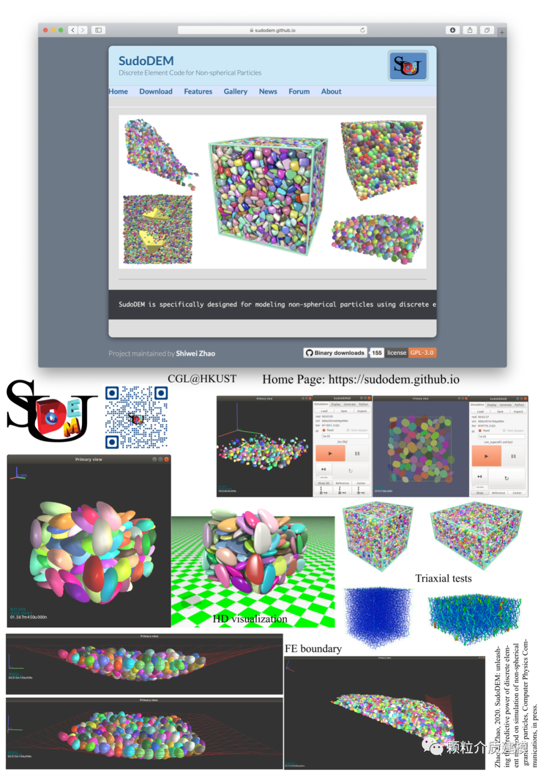
Preview in One Picture