Background
A brief introduction to the Material Point Method
The material point method (MPM) proposed by Sulsky et al. is one of the mesh-free approaches for coping with large deformation problems. The solution domain of the MPM is discretized and classified into Lagrangian (material Points) and Eulerian (background Grid) components. Moreover, the MPM calculation cycle is driven by mapping the kinematics and dynamics between the material points and background nodes.
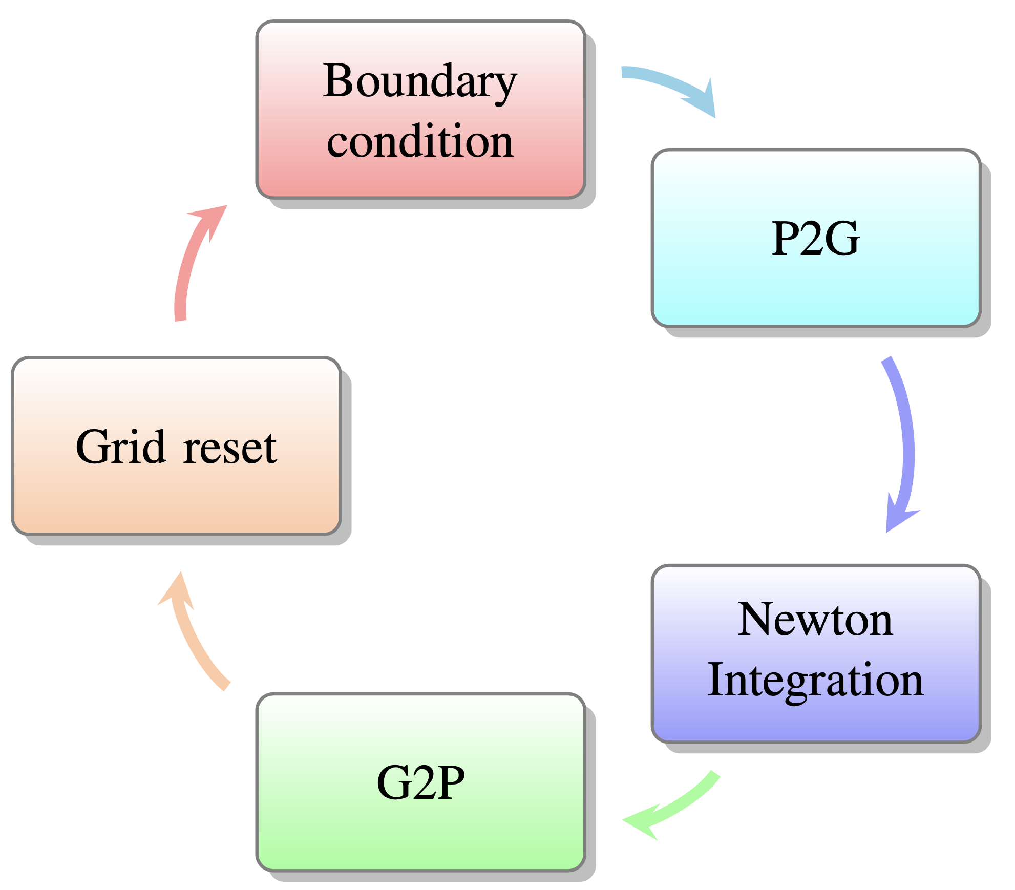
MPM calculation cycle within one timestep.
As shown in the Fig. \ref{fig:mpmloop}, five procedures will be conducted within one MPM iteration step.
-
Boundary condition (BC): the corresponding boundary condition will be applied to the material points or nodes, and the type of boundary condition can be: displacement BC, velocity BC, body force BC, traction force BC and temperature BC (if thermal task considered).
-
P2G: kinematic will be mapped from Particles to Grid nodes depends on the shape function. The kinematics consist of the mass, volume, moment, force/stress and the material field state variables including the volume gradient and displacement vector (if multi-material mode is activated).
-
Newton Integration: update the dynamics (moment and velocity) of background nodes using the kinematics expolated from the material points. Additional heat flux and temperature will be integrated once thermal task is run.
-
G2P: update all the state variables of material points assisted by the dynamics interpolated from background nodes. The calculation scheme of the stress and velocity/displacement of material points determined by the user-defined settings. For example, the stress update option governs if USF (Update Stress First) Bardenhagen or USL (Update Stress Late, Sulsky et al.) scheme will be executed. As for the velocity/position update, two options are also available as FLIP (FLuid Implicit Particle method, Brackbill and Ruppel) and PIC (Particle In Cell, Harlow). Moreover, the USF and mixture format of FLIP and PIC would be recommended by the authors.
-
Reset Grid: all the information of nodes will be reset. However, the state variable of material points will be transferred into the next step. The resetting process can avoid mesh distortion, which is why MPM can handle significant deformation problems.
MPM2D
MPM2D is designed to model large deformation problems employing the material point method. The whole program is written in C++ and further encapsulated by python to provide a user-friendly interface. Note that **GUI} utility is also developed and suggested for easily pre-processing and results rendering.
Minimal example python script for MPM2D-GUI is shown as follows:
An example for MPM2D-GUI python script.
## GUI settings for MPM2D
app.core.setAnalysisType(AnalysisType = "MPM")

## Some model settings

## Run the mpm simulation
app.run(1)
The framework of MPM2D
Five main classes are exposed to the python interface (Fig. \ref{fig:mpmframework}):
-
Analysis class is the core of MPM2D, it provides the platform for the communication among other members of MPM2D and navigates the whole simulation task.
-
Grid class depicts the geometry of the solution domain and maintains the hierarchical structure of elements and nodes.
-
Shape classes are responsible for the material points initialization and management. Clusters of the material points are created within a specific shape object. User-defined settings and boundary condition will not be assigned to the material points directly but is delegated to the functions of shapes instead.
-
Material classes affect the mechanical behaviour of material points. MPM2D supports the following material types: elastic material, Mohr-Coulomb material, Neo-Hookean material and Newton liquid.
-
Archiver class will dump the calculation result to a certain file format (binary or ASCII) as simple as possible to decrease the computation cost. When the simulation finishes, users can parse the raw results to the VTK file using the MPM2D extraction tool.
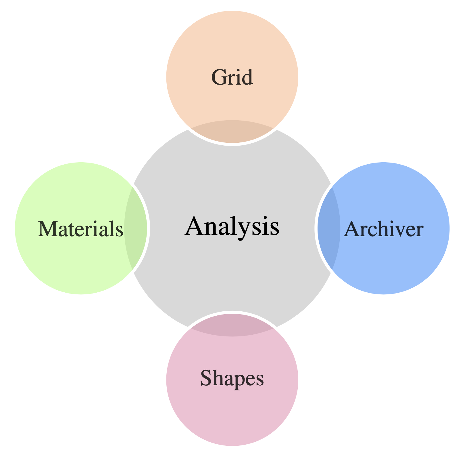
Framework of **MPM2D**.
The MPM2D GUI
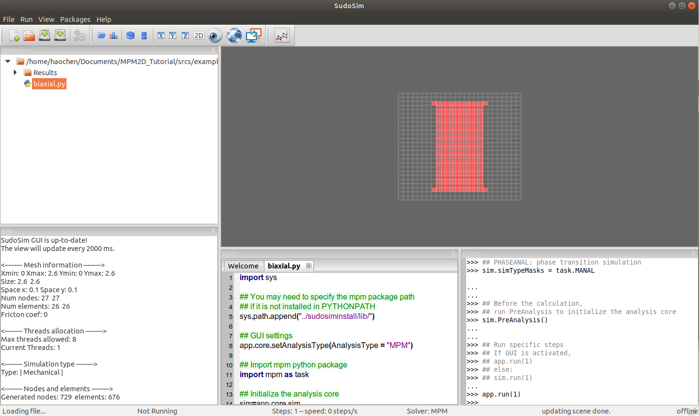
MPM2D GUI is always recommended to integrate with MPM tasks, and its snapshot is shown in Fig. \ref{fig:mpmgui}. Essential operation to run an MPM script is:
-
Click the button \includegraphics[scale=0.5]{open.png} and choose the directory path for the MPM script.
-
Double-click the target MPM script, e.g., the highlighted biaxial.py.
-
Click the gear button \includegraphics[scale=0.5]{run.png} and the MPM script has been pasted in the right-corner shell.
-
Type the command
app.run(1)at the right-corner shell to start the task.
Snapshot of the **MPM2D** GUI.