This the multi-page printable view of this section. Click here to print.
SudoDEM
- 1: Prerequisites
- 2: Examples
- 2.1: Example 0: run a simulation
- 2.2: Example 1: packing of super-ellipsoids
- 2.3: Example 2: triaxial tests of super-ellipsoids
- 2.4: Example 3: packing of GJKparticles
- 2.5: Example 4: packing of poly-superellipsoids
- 2.6: Example 5: packing of superellipses
- 3: Post-processing
- 4: Python Class Reference
1 - Prerequisites
A Linux distribution (Ubuntu 14 to 18 suggested) with Python 2.7 and some basic python packages (e.g., numpy) are assumed to have been installed at the users' side, but no other third-party packages (e.g., boost, qt) need installing.
Basic Linux Commands
Only several commands the users should know are enough to set off running a program. A terminal (i.e., command window) is open by pressing a shortcut ‘CTRL+ALT+T’ or whatever other operations.
-
sudo apt-get install package[^2] install a package to the system with root permission.
-
pwd: show the current path.
-
cd directory: change the directory to directory. The directory can be a relative or absolute path. Two special notations ‘.’ and ‘..’ denote the current directory and the parent directory, respectively, which are useful to type a relative path. For example, ' cd ../sub' will change the directory to the subdirectory ‘sub’ of the parent directory of the current path. ‘cd /home/user’ will change the directory to the absolute path ‘/home/user’.
-
prog or ./path/prog: run an executable named prog. If prog is exposed to the terminal, i.e., prog is in the searching path of the system, then just type the name prog like the command ‘cd’ at the last item; otherwise, a path should be specified to locate prog.
-
‘CTRL+C’: terminate a program at the terminal.
    $> sudo apt-get install python-numpy
    $> pwd
    $> cd /home/
    $> sudodem3d
Python 2.7
Python is sensitive to indent which is used to identify a script block. ‘#’ is used to comment a line which will not be executed. Here a piece of script is shown to explain the primitives of Python:
|
|
Ok, that is all you need to know prior to running a simulation. There are also other further techniques you might be interested in, e.g., how to open/read/write/close a file, and how to write a Python script with the object-oriented programming, which will be roughly introduced in the examples of this tutorial.
Package Setup
The project of SudoDEM is hosted on the website. Two ways to get the package installed are provided:
Binary Installation
Step 1: Get the package[^3]
Download the compiled package from the download page and unzip it to anywhere (e.g., /home/xxx/). If you just get a package of the main program which does not include the third-party libraries, then you need to download the package "3rdlibs.tar.xz" for the third-party libraries and extract it into the subfolder "lib". After that, make sure you get the following structure of folders:
::: {.forest} for tree= font=, grow'=0, child anchor=west, parent anchor=south, anchor=west, calign=first, inner xsep=7pt, edge path= (!u.south west) +(7.5pt,0) |- (.child anchor) pic folder ; , file/.style=edge path=(!u.south west) +(7.5pt,0) |- (.child anchor) ;, inner xsep=2pt,font= , before typesetting nodes= if n=1 insert before=[,phantom] , fit=band, before computing xy=l=15pt, [/home/xxx/SudoDEM/ [bin/ [sudodem3d] ] [lib/ [3rdlibs/] [sudodem/] ] [share/ ] ] :::
Step 2: Set the environmental variable PATH
Append the path of the executable sudodem3d, i.e., ‘/home/xxx/SudoDEM/bin’ to the environmental variable PATH by adding the following line to the config file ‘/home/xxx/.bashrc’:
PATH=${PATH}:/home/xxx/SudoDEM/bin
Non-root Compilation
Here is a video that may guide you to compile SudoDEM. You can copy the command lines directly from this video.
(1) Directory trees
After unzipping the source package, you have the following directory tree:
./home/xxx/SudoDEM
- [SudoDEM2D]
- [SudoDEM3D]
- [scripts]
- [INSTALL]
- [LICENSE]
- [Readme.md]
::: {.forest} for tree= font=, grow'=0, child anchor=west, parent anchor=south, anchor=west, calign=first, inner xsep=7pt, edge path= (!u.south west) +(7.5pt,0) |- (.child anchor) pic folder ; , file/.style=edge path=(!u.south west) +(7.5pt,0) |- (.child anchor) ;, inner xsep=2pt,font= , before typesetting nodes= if n=1 insert before=[,phantom] , fit=band, before computing xy=l=15pt, [/home/xxx/SudoDEM [SudoDEM2D ] [SudoDEM3D ] [scripts] [INSTALL,file ] [LICENSE,file ] [Readme.md,file ] ] :::
You may add subfolders, e.g.,‘3rdlib’, ‘build2d’, ‘build3d’, and ‘sudodeminstall’, inside the parent folder ‘SudoDEM’. Thus, the directory tree looks like
::: {.forest} for tree= font=, grow'=0, child anchor=west, parent anchor=south, anchor=west, calign=first, inner xsep=7pt, edge path= (!u.south west) +(7.5pt,0) |- (.child anchor) pic folder ; , file/.style=edge path=(!u.south west) +(7.5pt,0) |- (.child anchor) ;, inner xsep=2pt,font= , before typesetting nodes= if n=1 insert before=[,phantom] , fit=band, before computing xy=l=15pt, [/home/xxx/SudoDEM [SudoDEM2D ] [SudoDEM3D ] [3rdlib] [build2d] [build3d] [sudodeminstall] [scripts] [INSTALL,file ] [LICENSE,file ] [Readme.md,file ] ] :::
The subfolder ‘3rdlib’ is for the third-party libraries. Note that the subfolder ‘3rdlib’ hosts the header files and the compiled dynamic libraries, while for launching SudoDEM you need to copy all dynamic libraries ‘*.so.*’ files into the install directory, e.g., ‘lib/3rdlibs/’. The compilation of the 2D and 3D versions will be done within the subfolders ‘build2d’ and ‘build3d’, respectively. The compiled outputs (binary and library) will be installed in the subfolder ‘sudodeminstall’.
(2) Compilation of third-party libraries
::: {.forest} for tree= font=, grow'=0, child anchor=west, parent anchor=south, anchor=west, calign=first, inner xsep=7pt, edge path= (!u.south west) +(7.5pt,0) |- (.child anchor) pic folder ; , file/.style=edge path=(!u.south west) +(7.5pt,0) |- (.child anchor) ;, inner xsep=2pt,font= , before typesetting nodes= if n=1 insert before=[,phantom] , fit=band, before computing xy=l=15pt, [/home/xxx/SudoDEM/3rdlib [boost-1_6_7] [eigen3.3.5] [libQGLViewer-2.6.3] [minieigen] ] :::
Four major libraries:
-
Boost-1.67
Download the source from its official page (https://www.boost.org/users/history/version_1_67_0.html) or the github repo (https://github.com/SwaySZ/boost-1_6_7).cd boost-1\_6\_7 ./bootstrap.sh --prefix=$PWD/../boost167 --with-libraries=python,thread,filesystem,iostreams,regex,serialization,system,date_time link=shared runtime-link=shared --without-icu ./b2 -j3 ./b2 install -
Eigen-3.3.5: no need to compile but all head files will be included. You may download the source from the repo (https://github.com/SwaySZ/Eigen-3.3.5).
-
MiniEigen
Download the source from the repo (https://github.com/SwaySZ/minieigen). Set the directory of your compiled boost in the file ‘CMakeLists.txt’:set(BOOST_ROOT "/home/swayzhao/software/DEM/3rdlib/boost167")Then,
mkdir build
cd build
cmake ../
make
After compilation, you will get the shared library ‘minieigen.so’. Copy it to the folder ‘lib/3rdlibs/py’.
-
LibQGLViewer-2.6.3
Download the source from the repo (https://github.com/SwaySZ/libQGLViewer-2.6.3)cd QGLViewer qmake make
Tools and dependencies:
-
biuld-essential, cmake
-
freeglut3-dev
-
zlib1g-dev (boost)
-
python-dev (boost)
-
pyqt4-dev-tools
-
qt4-default
-
python-numpy python-tk
-
libbz2-dev
-
python-xlib python-qt4
-
ipython3.0 python-matplotlib
-
libxi-dev
-
libglib2.0-dev
-
libxmu-dev
(3) Compilation of SudoDEM main programs
Here we show the example to compile SudoDEM3D as follows. In the folder ‘SudoDEM3D’, you have the directory tree:
::: {.forest} for tree= font=, grow'=0, child anchor=west, parent anchor=south, anchor=west, calign=first, inner xsep=7pt, edge path= (!u.south west) +(7.5pt,0) |- (.child anchor) pic folder ; , file/.style=edge path=(!u.south west) +(7.5pt,0) |- (.child anchor) ;, inner xsep=2pt,font= , before typesetting nodes= if n=1 insert before=[,phantom] , fit=band, before computing xy=l=15pt, [/home/xxx/SudoDEM/SudoDEM3D [cMake] [CMakeLists.txt, file] [core] [doc] [gui] [lib] [pkg] [py] ] :::
Prior to compiling, you may need to edit the file ‘CMakeLists.txt’, in which you may change the installation directory, paths of library header files, etc.
(a) The installation path is set by
SET(CMAKE_INSTALL_PREFIX "${CMAKE_CURRENT_SOURCE_DIR}/../sudodeminstall/SudoDEM3D")
(b) The root directory of BOOST library is set by
set(BOOST_ROOT "${CMAKE_CURRENT_SOURCE_DIR}/../3rdlib/boost167")
(c) For the QGLViewer, the paths for both header files and library are set by the following two lines:
set(QGLVIEWER_INCLUDE_DIR "${CMAKE_CURRENT_SOURCE_DIR}/../3rdlib/libQGLViewer-2.6.3/")
set(QGLVIEWER_LIBRARIES "${CMAKE_CURRENT_SOURCE_DIR}/../3rdlib/libQGLViewer-2.6.3/QGLViewer/libQGLViewer.so")
(d) Copy your system-installed numpy and pyqt4 to the path ‘./lib/3rdlibs/py’. You may also change the search path of numpy in the file FindNumPy.cmake under the folder ‘cMake’:
set(DPDIR "${CMAKE_CURRENT_SOURCE_DIR}/../dem2dinstall/SudoDEM/lib/3rdlibs/py/")
Compile and install SudoDEM3D:
cd build3d
cmake ../SudoDEM3D
make -j3
make install
The binary ‘sudodem3d’ will be installed in the path ‘/home/xxx/SudoDEM/sudodeminstall/SudoDEM3D/bin/’. Append the path to the environmental variable PATH by adding the following line to the config file ‘/home/xxx/.bashrc’:
PATH=${PATH}:/home/xxx/SudoDEM/sudodeminstall/SudoDEM3D/bin
You are expected to get the following directory tree after installation:
::: {.forest} for tree= font=, grow'=0, child anchor=west, parent anchor=south, anchor=west, calign=first, inner xsep=7pt, edge path= (!u.south west) +(7.5pt,0) |- (.child anchor) pic folder ; , file/.style=edge path=(!u.south west) +(7.5pt,0) |- (.child anchor) ;, inner xsep=2pt,font= , before typesetting nodes= if n=1 insert before=[,phantom] , fit=band, before computing xy=l=15pt, [/home/xxx/SudoDEM/sudodeminstall [bin ] [lib [3rdlibs [*.so,file] [py [minieigen.so,file] [numpy] [PyQt4] [other Python modules,file] ] ] [sudodem] ] [share] ] :::
Note: the installation procedure of SudoDEM will overwrite the above directories except ‘3rdlibs’. You need to copy all the 3rd-party libraries compiled above (boost, libQGLViewer, minieigen) to ‘3rdlibs’. If you encounter any problems about the 3rd-libraries, you may check the directory tree for the binary package of SudoDEM.
IMPORTANT: Add rpath to all 3rd-party libraries under ‘3rdlibs’ by executing the script ‘changerpath.sh’ in the folder ‘scripts’.
cd 3rdlibs
cp /home/xxx/SudoDEM/scripts/changerpath.sh .
chmod +x changerpath.sh
./changerpath.sh
Note: ‘changerpath.sh’ will add rpath ‘$ORIGIN’ to all dynamic libraries under ‘3rdlibs’ and rpath ‘$ORIGIN/../../’ to all dynamic libraries under ‘3rdlibs/py/PyQt4’. An rpath would make a dynamic library to search its dependencies (other dynamic libraries) from the rpath-specified path in the first place, which helps to avoid invoking other versions of dependencies in the system path.
2 - Examples
We prepared several examples to show a quick start of using SudoDEM, and the corresponding script for each example is available on the website or the Github repository (https://github.com/SwaySZ/ExamplesSudoDEM).
2.1 - Example 0: run a simulation
This example will show the ingredients of a simulation by simulating a sphere free falling onto a ground. We prepare a Python script named ‘example0.py’ at our work directory (e.g., /home/xxx/example'). Open a terminal, and type ‘sudodem3d example0.py’ if the work directory is at ‘/home/xxx/example/’ otherwise providing a relative or absolute path of ‘example0.py’.
Here is the script of ‘example0.py’:
|
|
Run the simulation by typing the following command in a terminal:
sudodem3d example0.py
For multi-threads, e.g., using 2 threads [^4]
sudodem3d -j2 example0.py
The recorded data ‘data.dat’ looks like below:
iter, x, y, z
10000 0.0 0.0 9.95588676912
20000 0.0 0.0 9.82357353912
30000 0.0 0.0 9.60306030912
40000 0.0 0.0 9.29434707912
50000 0.0 0.0 8.89743384912
60000 0.0 0.0 8.41232061912
70000 0.0 0.0 7.83900738912
We can take a quick view on the recorded data using gnuplot. Install gnuplot by typing the following command in a terminal:
sudo apt install gnuplot
Then, open gnuplot and plot the data as shown in Fig. 3.1{reference-type=“ref” reference=“figsinglesp”}:
$> gnuplot
    gnuplot> plot 'data.dat' using ($1/10000):4; set xlabel 'iterations [x10000]'; set ylabel 'position z [m]'
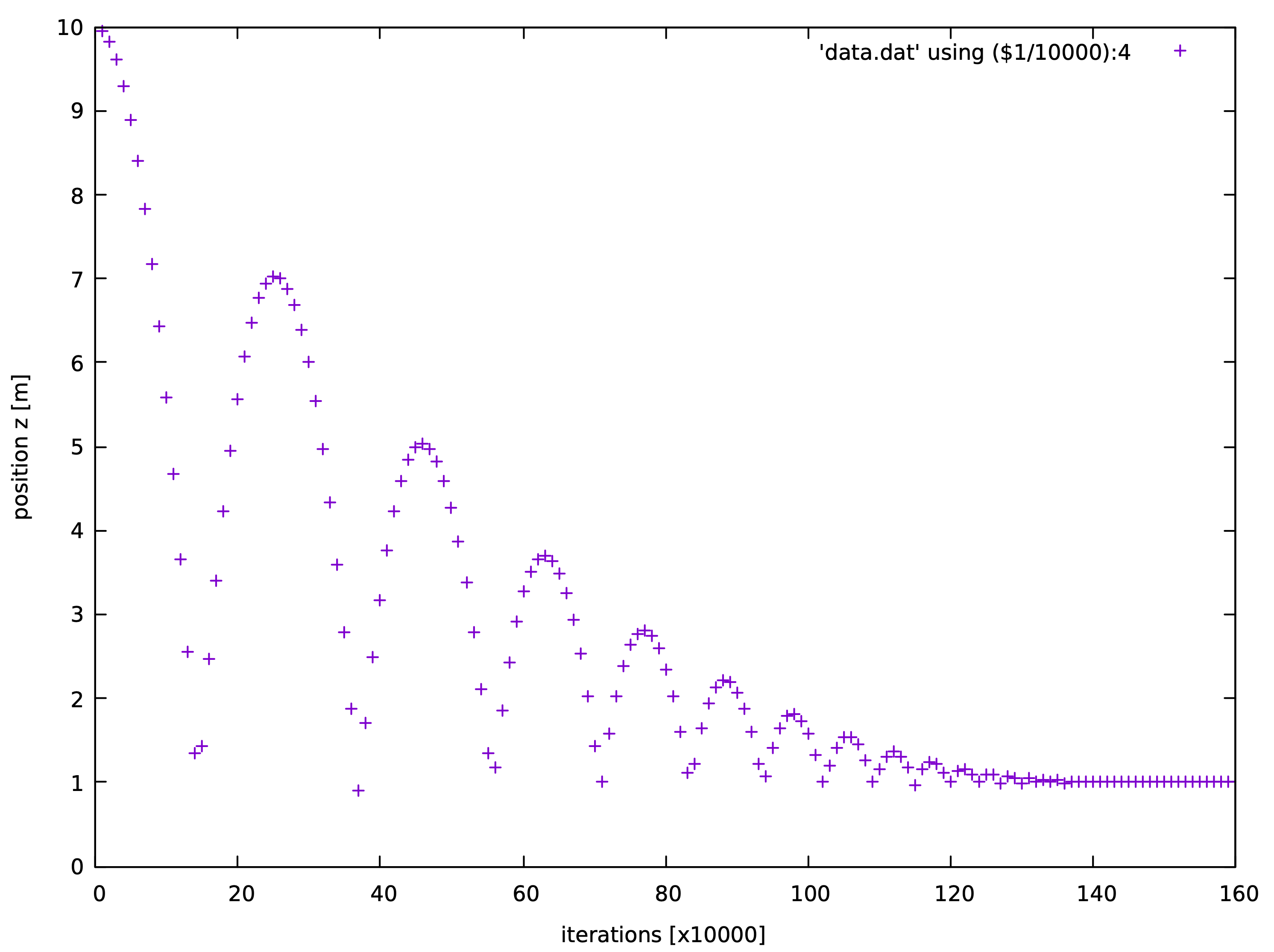
The z-position of a sphere free falling onto a ground.
2.2 - Example 1: packing of super-ellipsoids
The surface function of a superellipsoid in the local Cartesian coordinates can be defined as $$\label{eqsurface} \Big(\big|\frac{x}{r_x}\big|^{\frac{2}{\epsilon_1}} + \big|\frac{y}{r_y}\big|^{\frac{2}{\epsilon_1}}\Big)^{\frac{\epsilon_1}{\epsilon_2}} + \big|\frac{z}{r_z}\big|^{\frac{2}{\epsilon_2}} = 1$$ where $r_x, r_y$ and $r_z$ are referred to as the semi-major axis lengths in the direction of x, y, and z axies, respectively; and $\epsilon_i (i=1,2)$ are the shape parameters determining the sharpness of particle edges or squareness of particle surface. Varying $\epsilon_i$ between 0 and 2 yields a wide range of convex-shaped superellipsoid. Two functions for generating a superellipsoid are highlighted below (see Sec. 5.1.2{reference-type=“ref” reference=“modsuperquadrics”}):
-
NewSuperquadrics2($r_x$, $r_y$, $r_z$, $\epsilon_1$, $\epsilon_2$, mat, rotate, isSphere)
-
NewSuperquadrics_rot2($r_x$, $r_y$, $r_z$, $\epsilon_1$, $\epsilon_2$, mat, $q_w$, $q_x$, $q_y$, $q_z$, isSphere)
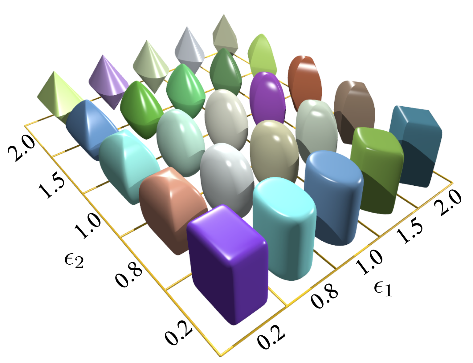
Superellipsoid.
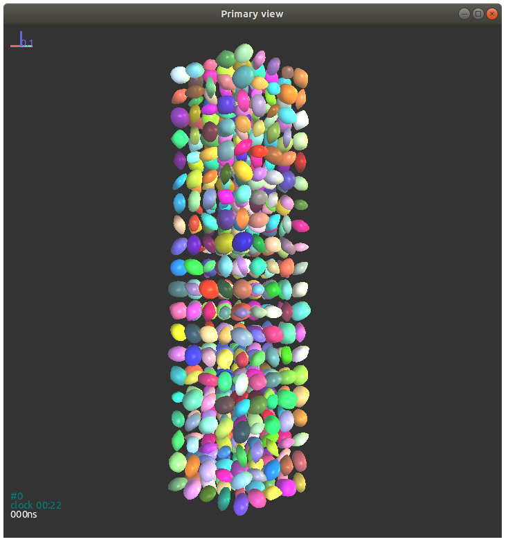
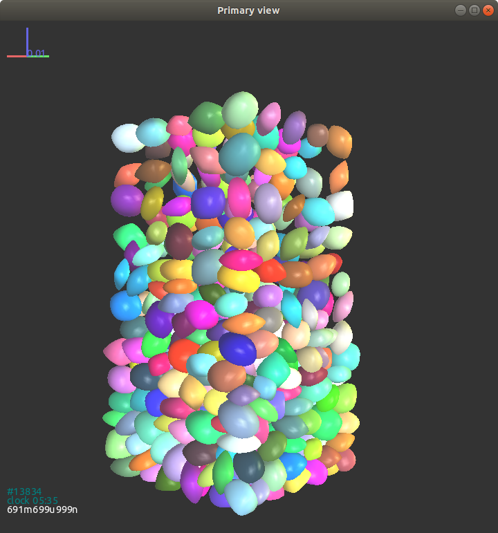
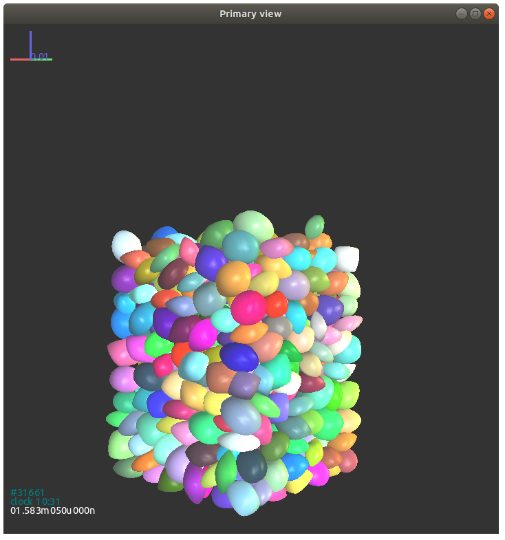
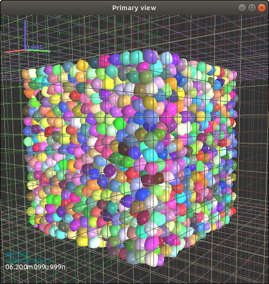
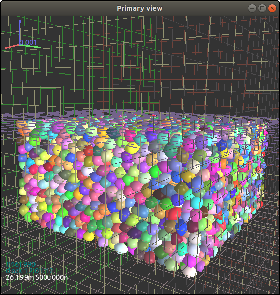
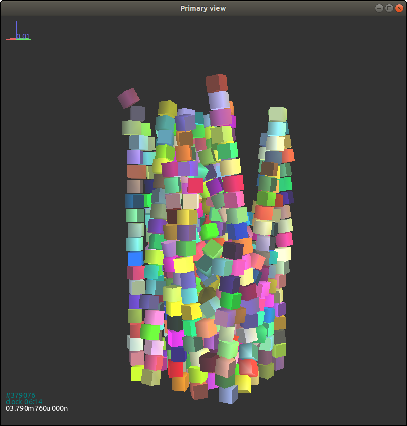
Here we give an example of a simulation of superellipsoids free falling into a cubic box.
|
|
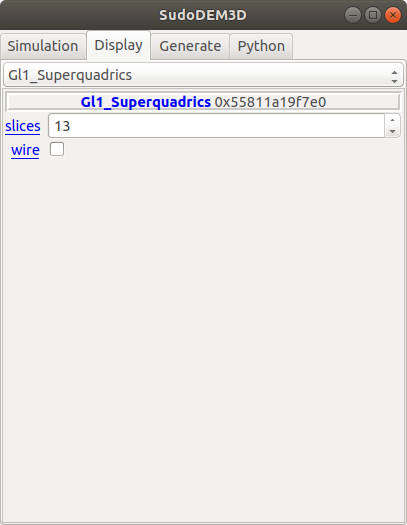
With a GUI controller, we can click ‘show 3D’ button at the panel ‘Simulation’ to display the simulating scene. On the ‘Display’ panel, select the render ‘Gl1_Superquadrics’ to configure the resolution of solid or wireframe particles, as shown in Fig. 3.3{reference-type=“ref” reference=“figguidisplay”}.
Figs. 3.4{reference-type=“ref” reference=“figexp11”} - 3.6{reference-type=“ref” reference=“figexp13”} show simulations of packing of superellipsoids at different states for the presented example.
Several properties and methods for a shape Superquadrics are listed below:
-
Properties:
-
$r_x$, $r_y$, $r_z$: float, semi-major axis lengths in x, y, and z axies.
-
$\epsilon_1$, $\epsilon_2$: float, shape parameters.
-
isSphere: bool, particle is spherical or not.
-
-
Methods:
-
getVolume(): float, return particle’s volume.
-
getrxyz(): Vector3, return particle’s rxyz.
-
geteps(): Vector2, return particle’s eps1 and eps2.
-
Here is an example to get the volume of a particle with an id of 100:
volume = O.bodies[100].shape.getVolume()
A general method to list all properties of an object is as follows:
O.bodies[100].dict()
The output is like follows:
{'bound': <Aabb instance at 0x56072ec83da0>,
 'chain': -1,
 'clumpId': -1,
 'flags': 3,
 'groupMask': 1,
 'id': 100,
 'iterBorn': 0,
 'material': <SuperquadricsMat instance at 0x56072e6ed5f0>,
 'shape': <Superquadrics instance at 0x56072ec83b60>,
 'state': <State instance at 0x56072ec839e0>,
 'timeBorn': 0.0}
We can see that the properties are printed in a dict form. Note that the value enclosed by pointy brackets is another object (actually, instance of an object with a specified memory address), which means that we can further access it using the ".dict()" method. Again, the properties of the object State can be accessed by:
O.bodies[100].state.dict()
The output is as follows:
{'angMom': Vector3(0,0,0),
 'angVel': Vector3(0,0,0),
 'blockedDOFs': 0,
 'densityScaling': 1.0,
 'inertia': Vector3(0.0045389863901528615,0.007287422614611933,
                           0.0067053718092146865),
 'isDamped': True,
 'mass': 3.225715855242557,
 'refOri': Quaternion((1,0,0),0),
 'refPos': Vector3(0,0,0),
 'se3': (Vector3(0,0.8,3),
  Quaternion((0.3970010520699211,0.5339678220536823,
                     -0.7465042060609055),2.1754719537556495)),
 'vel': Vector3(0,0,0)}
For an object Shape, we list all properties which may vary for different child classes.
O.bodies[100].shape.dict()
The output is as follows:
{'color': Vector3(0.6407663308273844,0.07426042997942327,
                            0.05872324344642611),
 'eps': Vector2(1.3975848801318045,1.5376309088540607),
 'eps1': 1.3975848801318045,
 'eps2': 1.5376309088540607,
 'highlight': False,
 'isSphere': False,
 'rx': 0.1,
 'rxyz': Vector3(0.1,0.06469580193313924,0.07572423080016706),
 'ry': 0.06469580193313924,
 'rz': 0.07572423080016706,
 'wire': False}
Here we give an example to list ids and positions of all superellipsoids:
for b in O.bodies: # loop all bodies in the simulation
    # we have to check if the present body is a superellipsoid or others, e.g., a wall
    if isinstance(b.shape, Superquadrics): # if it is a superellipsoid, then to do
        pid = b.id # get the id of particle b
        pos = b.state.pos # get the position of particle b
        print pid, pos
2.3 - Example 2: triaxial tests of super-ellipsoids
This example shows a triaxial compression simulation of superellipsoids using an Engine CompressionEngine. The users can also customized their engines or compression procedures easily via a PyRunner Engine. Here is a basic setup of CompressionEngine for consolidation and compression below.
-
Consolidation
1 2 3 4 5 6 7 8 9 10 11 12 13 14 15triax=CompressionEngine( goalx = 1.0e5, # confining stress 100 kPa goaly = 1.0e5, goalz = 1.0e5, savedata_interval = 10000, echo_interval = 2000, continueFlag = False, max_vel = 100.0, gain_alpha = 0.5, f_threshold = 0.01, #1-f/goal fmin_threshold = 0.01, #the ratio of deviatoric stress to mean stress unbf_tol = 0.01, #unblanced force ratio file='record-con' )-
goalx = goaly = goalz = confining stress
-
savedata_interval: the interval of DEM iterations for saving some data (Axial Strain, Volumetric Strain, Mean Stress and DeviatorStress) into a file specified by file. Deprecated for consolidation.
-
echo_interval: the interval of DEM iterations for outputting information (Iterations, Unbalanced force ratio, stresses in x, y, z directions) in the terminal
-
continueFlag: reserved keyword for continuing consolidation or compression.
-
max_vel: the maximum velocity of a wall, which is useful to constrain the movement of a wall during confining.
-
gain_alpha $\alpha$: guiding the movement of the confining walls. $$v_w = \alpha \frac{f_w - f_g}{\Delta t \sum k_n}$$ where $v_w$ is the velocity of a confining wall at the next time step; $f_w$ and $f_g$ are the present and goal confining forces, respectively; $\Delta t$ is the time step, and $\sum k_n$ is the summation of normal contact stiffness from all particle-wall contacts on this wall.
-
f_threshold $\alpha_f$: a target ratio of the deviation of the present stress from the goal to the goal, i.e., $$\alpha_f = \frac{|f_w-f_g|}{f_g}$$
-
fmin_threshold $\beta_f$: a target ratio of the deviatoric stress $q$ to the mean stress $p$, i.e., $$\beta_f = \frac{q}{p},\quad p= \frac{\sigma_{ii}}{3},\quad q=\sqrt{\frac{3}{2}\sigma_{ij}^{'}\sigma_{ij}^{'}}$$ $$\sigma_{ij} = \frac{1}{V}\sum_{c\in V}f_i^cl_j^c,\quad \sigma_{ij}^{'}=\sigma_{ij}-p\delta_{ij}$$ where $\sigma_{ij}$ is the stress tensor with an assembly, and $\sigma_{ij}^{'}$ is its corresponding deviatoric part; $V$ is the total volume of the specimen; $f^c$ and $l^c$ are the contact force and branch vector at contact $c$, respectively, and $\delta_{ij}$ is the Kronecker delta.
-
unbf_tol $\gamma_f$: a target unbalanced force ratio defined as $$\gamma_f = \frac{\sum\limits_{B_i\in V} |\sum\limits_{j\in B_i}f^c_j+f^b_j|}{2\sum\limits_{c\in V}|f^c|}$$ Note: the consolidation ends up with that all $\alpha_f$, $\beta_f$ and $\gamma_f$ reach the targets.
-
file: the file name for the recording file
-
-
Compression
1 2 3 4 5 6 7 8 9 10 11 12 13 14 15 16triax=CompressionEngine( z_servo = False, goalx = 1.0e5, goaly = 1.0e5, goalz = 0.01, ramp_interval = 10, ramp_chunks = 2, savedata_interval = 1000, echo_interval = 2000, max_vel = 10.0, gain_alpha = 0.5, file='sheardata', target_strain = 0.4, gain_alpha = 0.5 )-
z_servo: a False value will trigger a strain (or displacement) control in the z direction, and in this case goalz needs a strain rate.
-
ramp_interval: iterations needed for reaching a constant strain rate. This keyword is designed to mimic a continuing loading at laboratory, but it seems not too valued and setting a small value to kindly deprecate it.
-
ramp_chunks: number of intervals to reach the constant strain rate combined with the keyword ramp_interval. It will be deprecated as does ramp_interval.
-
target_strain: at this level of strain the shear procedures ends. The strain is ogarithmic strain.
Note: to ensure quasi-static behavior during shear, the shear strain rate should be sufficiently small. Specifically, the inertial number $I$ should be maintained less than $10^{-3}$ $$I = \dot{\epsilon_1}\frac{\hat{d}}{\sqrt{\sigma_0/\rho}}$$ where $\dot{\epsilon_1}=\mathrm{d}\epsilon_1/\mathrm{d}t$ is the major principal strain rate; $\hat{d}$ and $\rho$ are the average diameter and material density of particles respectively; $\sigma_0$ is the confining stress.
-
As a demonstration, we first give an example of consolidation as follows:
|
|
The output in the terminal is akin to the follows:
calm procedure is over
0 particles are deleted!
consolidation begins
Iter 50000 Ubf 0.483161, Ss_x:9.67986e-05, Ss_y:4.15364e-05, Ss_z:6.1184e-05, e:0.992618
Iter 52000 Ubf 0.461741, Ss_x:1.2412, Ss_y:1.06812, Ss_z:1.10116, e:0.854445
Iter 54000 Ubf 0.263699, Ss_x:1.75334, Ss_y:1.98567, Ss_z:1.62181, e:0.757469
Iter 56000 Ubf 0.118329, Ss_x:3.06302, Ss_y:3.54818, Ss_z:3.22986, e:0.679106
Iter 58000 Ubf 0.0110747, Ss_x:22.0177, Ss_y:21.3303, Ss_z:21.3485, e:0.614824
Iter 60000 Ubf 0.000577066, Ss_x:91.4199, Ss_y:89.6039, Ss_z:89.1057, e:0.58984
Iter 62000 Ubf 0.000128293, Ss_x:100.012, Ss_y:99.7251, Ss_z:99.6123, e:0.587807
consolidation completed!
After consolidation (see the snapshot in Fig. 3.7{reference-type=“ref” reference=“figex2consol”}), we obtain a state file by
|
|
Then, the consolidated assembly is subjected to triaxial compression with the following scripts.
|
|
The compression ends up with an axial strain of 40%, and the final configuration of particles is shown in Fig. 3.8{reference-type=“ref” reference=“figex2shear”}.
The macroscopic mechanical response of a granular material during shearing can be quantified by the stress tensor that is calculated from discrete measurements with the following definition: $$\label{eqDEMstress} \sigma_{ij} = \frac{1}{V} \sum_{c \in V} f_i^c l_j^c$$ where $V$ is the total volume of the assembly, $f^c$ is the contact force at the contact $c$, and $l^c$ is the branch vector joining the the centres of the two contacting particles at contact $c$. The mean stress $p$ and the deviatoric stress $q$ are defined as: $$p = \frac{1}{3}\sigma_{ii},\quad q = \sqrt{\frac{3}{2} \sigma_{ij}^{'}\sigma_{ij}^{'}}$$ where $\sigma_{ij}^{'}$ is the deviatoric part of stress tensor $\sigma_{ij}$.
Given that the cubical specimens are confined by rigid walls, the axial strain $\epsilon_z$ and the volumetric strain $\epsilon_v$ can be approximately calculated from the positions of the boundary walls, i.e., $$\epsilon_z = \int_{H_0}^{H}\frac{\mathrm{d}h}{h}=-\ln\frac{H_0}{H},\quad \epsilon_v = \epsilon_x+\epsilon_y+\epsilon_z=\int_{V_0}^{V}\frac{\mathrm{d}v}{v}=-\ln\frac{V_0}{V}$$ where $H$ and $V$ are the height and volume of the specimen during shearing, respectively, and $H_0$ and $V_0$ are their initial values before shear. Positive values of volumetric strain represent dilatancy.
The recorded data ‘sheardata’ looks like below:
AxialStrain VolStrain meanStress deviatorStress
0.000511000266 0.000490480823 106090.98 15931.56
0.003011001516 0.002450117535 131061.41 85718.91
0.005511002766 0.003867756447 148076.65 131980.95
0.008011004016 0.004825115794 159924.28 163706.90
0.010511005266 0.005409561745 168606.27 186520.14
0.013011006516 0.005673777079 175131.53 203243.28
0.015511007766 0.005650846281 180293.19 216248.17
0.018011009016 0.005393122254 184581.23 227010.23
Then we can plot the stress-strain variation and the loading path as shown in Figs. 3.9{reference-type=“ref” reference=“figex2shearstress”} and 3.10{reference-type=“ref” reference=“figex2shearpath”}.
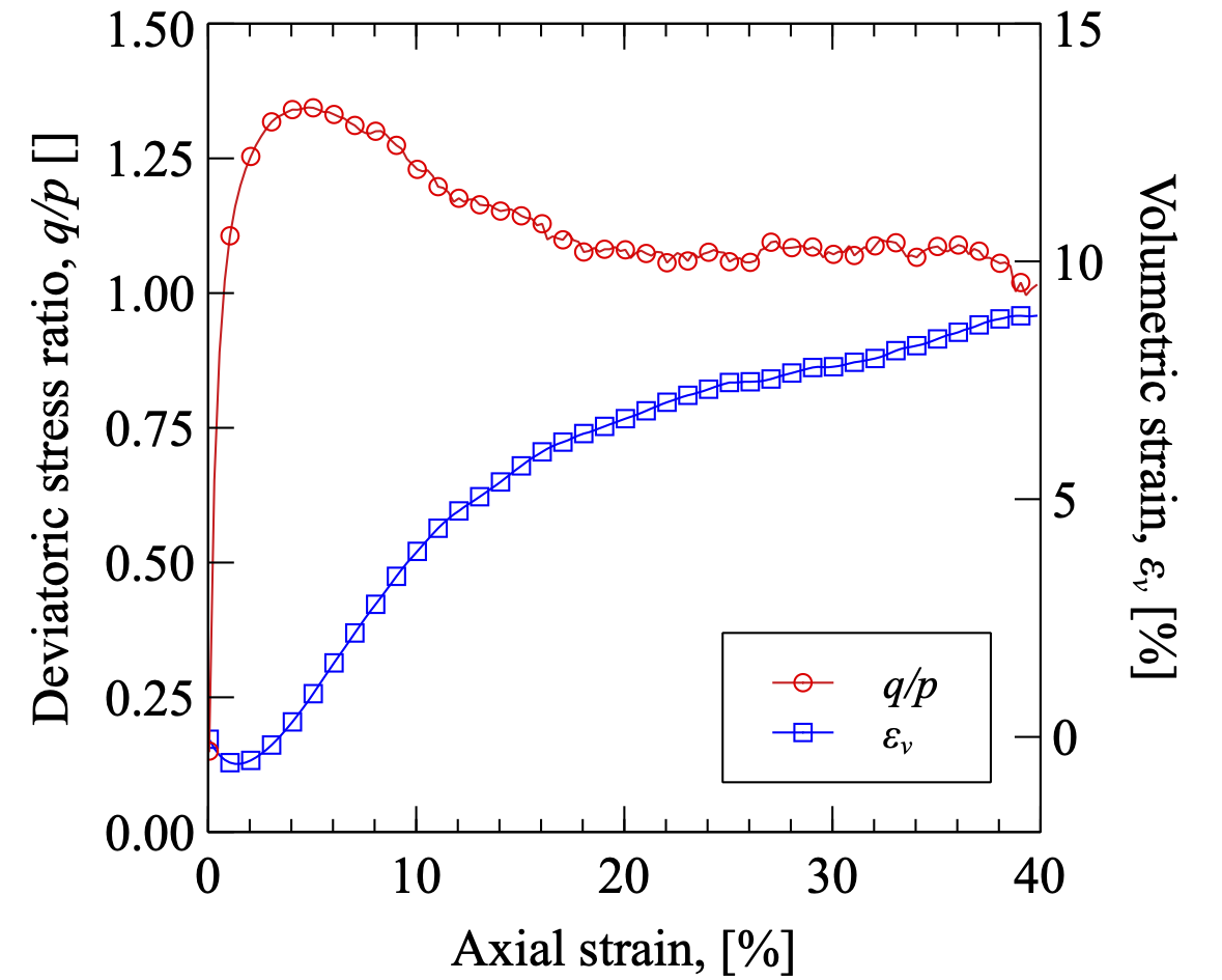
Shearing.
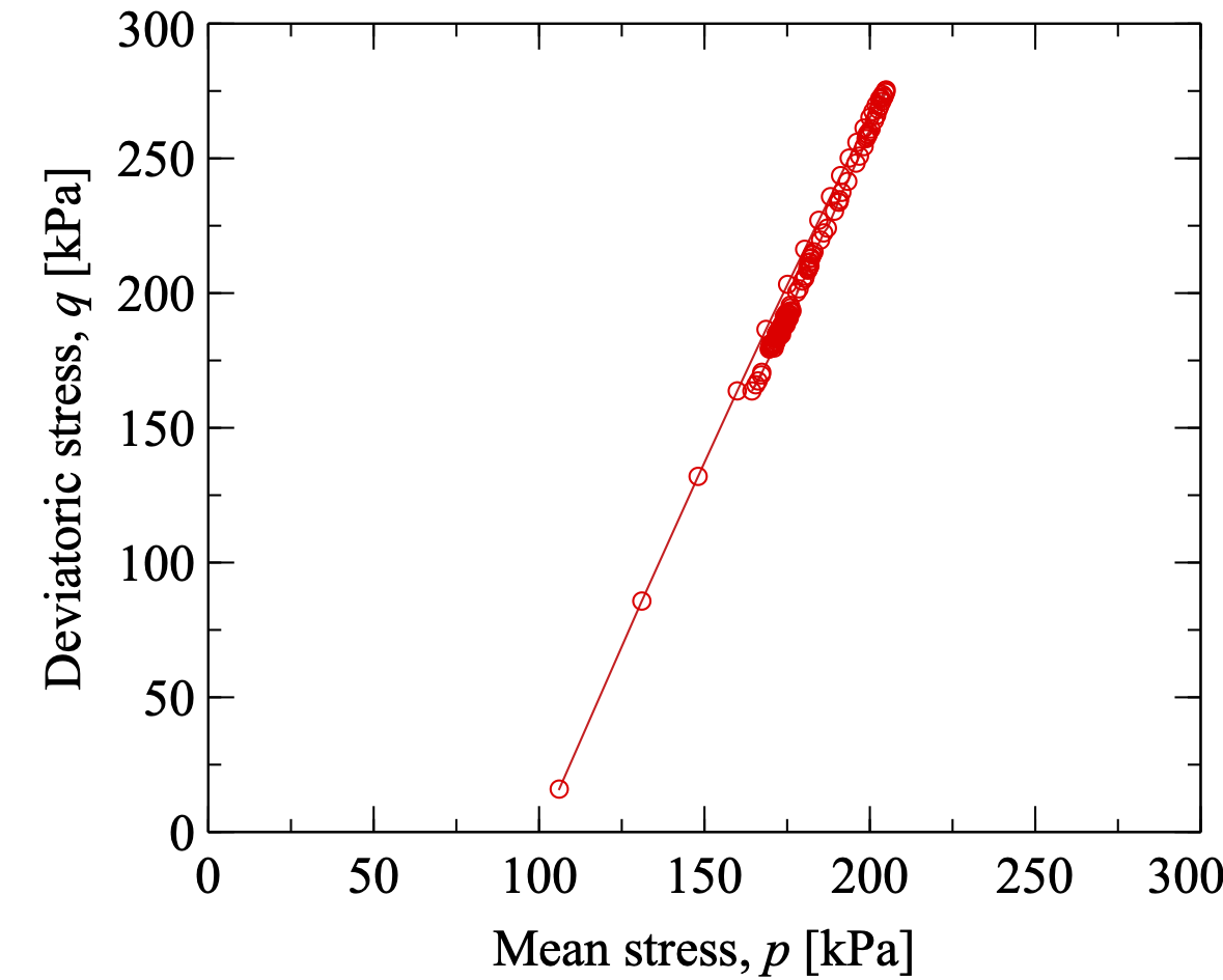
Loading path during shearing.
During shearing, a series of states (i.e., files "shearxxx.xml.bz2") has been saved sequentially so that it is readily to access other data for post-processing, e.g., variation of mean coordination number, anisotropy and so forth.
2.4 - Example 3: packing of GJKparticles
There are five kinds of shapes, namely sphere, polyhedron, cone, cylinder and cuboid, in SudoDEM, for which the GJK algorithm of contact detection is performed [^5], so that we coined a name GJKparticle for grouping these particle shapes. In the Python module _gjkparticle_utils (see Sec. 5.1.3{reference-type=“ref” reference=“modgjkparticle”}), several construction functions are provided including:
-
GJKSphere(radius,margin,mat)
-
GJKPolyhedron(vertices,extent,margin,mat, rotate)
-
GJKCone(radius, height, margin, mat, rotate)
-
GJKCylinder(radius, height, margin, mat, rotate)
-
GJKCuboid(extent, margin,mat, rotate)
Note: a margin is used to expand a particle for achieving a better computational efficiency, which however should be large enough for ensuring that collision occurs in this small region but small enough for shape fidelity.
Similar to Example 1, we conduct some simulations of particles free falling into a cubic box. We first import some modules:
|
|
Next, define some constants:
|
|
Define a lattice grid:
|
|
Set properties of materials:
|
|
Create the cubic box:
|
|
Define engines and set a fixed time step:
|
|
Polyhedral particles are generated as follows:
|
|
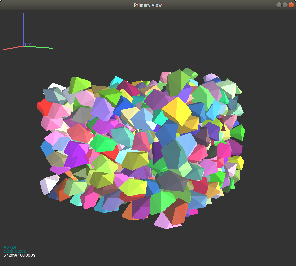 {#figgjkpolyhedron width=“8cm”}
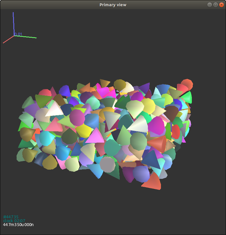
 {#figgjkcone width=“8cm”}
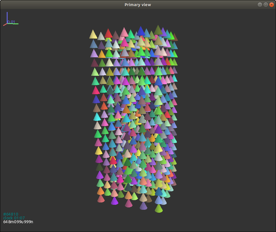
For cones, we change the GenSample functions as follows:
|
|
Fig. 3.12{reference-type=“ref” reference=“figgjkcone”} shows final packing of cones without random initial orientations (i.e., the argument rotate is False). It can be seen that particles still align in the lattice grid due to no disturbance in the tangential direction.
Set the argument rotate to True as follows:
|
|
 {#figgjkcone2 width=“8cm”}
Rerun the simulation, and the initial particles have random orientations. After free falling under gravity, it can be seen that the lattice alignment corrupts, referring to Fig. 3.13{reference-type=“ref” reference=“figgjkcone2”}
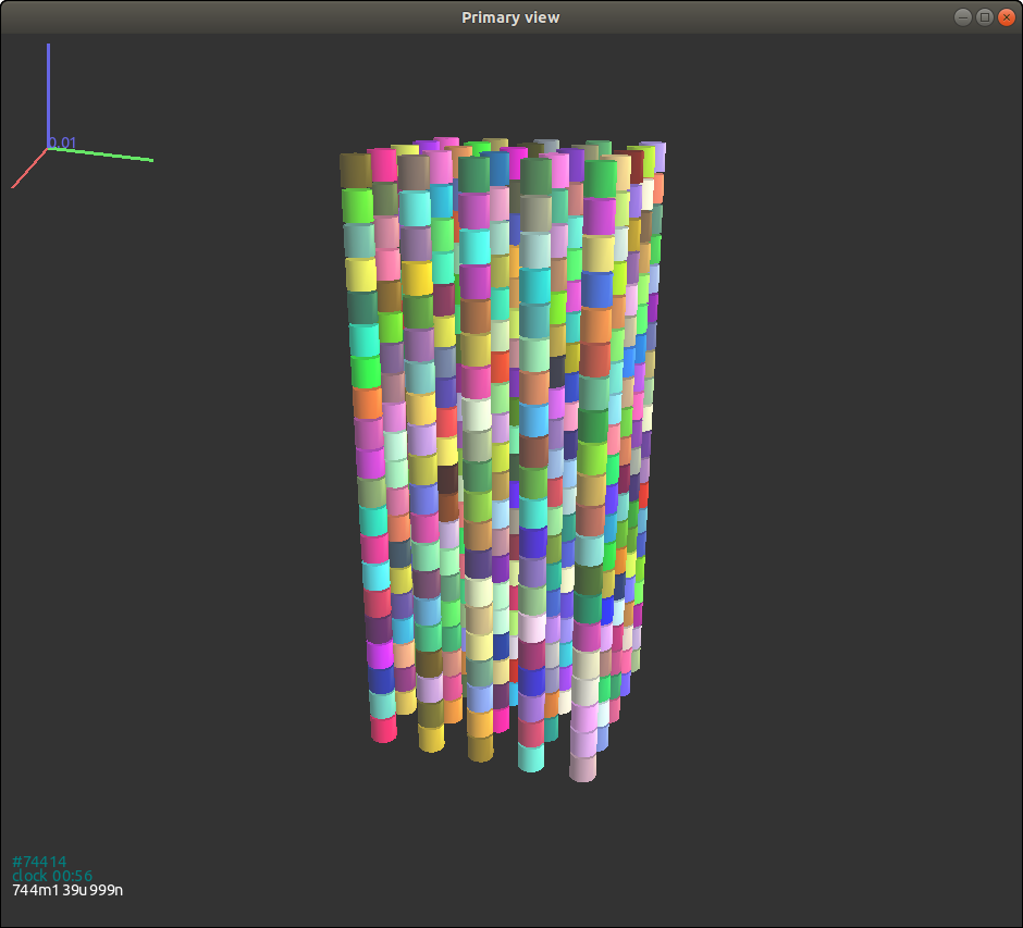 {#figgjkcylinder width=“8cm”}
For cylindrical particles, the function GenSample is replaced as follows:
|
|
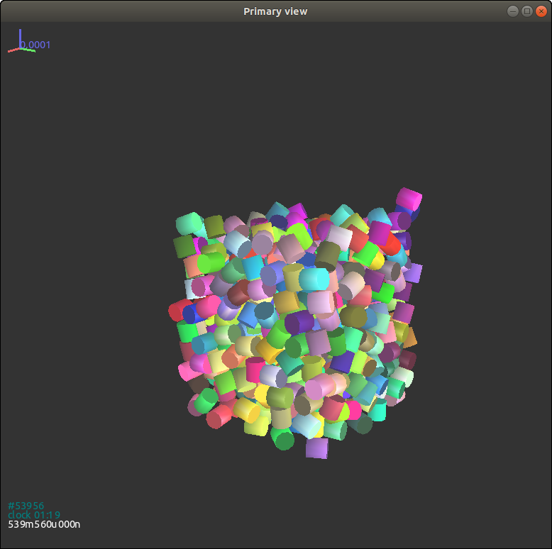 {#figgjkcylinder2 width=“8cm”}
Rerun the simulation, we obtain final packing of cylindrical particles as shown in Fig. 3.14{reference-type=“ref” reference=“figgjkcylinder”}, where it is evident that all particles stay in a lattice grid after free falling. Again, we reset the argument rotate to True so that all initial particles will have random orientations.
|
|
Rerun the simulation again, the column of cylindrical particles collapse into the cubic box. The final state is visualized in Fig. 3.15{reference-type=“ref” reference=“figgjkcylinder2”}.
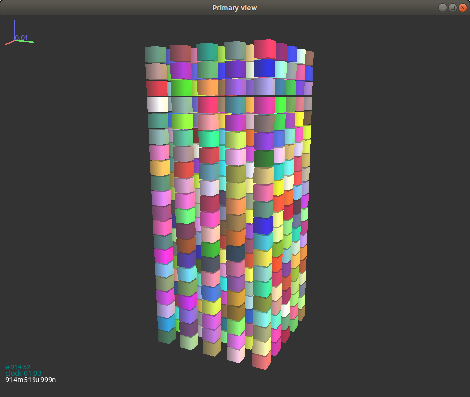 {#figgjkcuboid width=“8cm”}
 {#figgjkcuboid2 width=“8cm”}
We then continue two more simulations of cuboids. Change the function GenSample as follows:
|
|
We obtain the final packing of cuboids without initial random orientations as shown in Fig. 3.16{reference-type=“ref” reference=“figgjkcuboid”}. Again, the alignment of particles remains a lattice form. Rerun the simulation with the argument rotate setting to True as follows:
|
|
The column of particles collapses but not too much due to small gaps between particles.
2.5 - Example 4: packing of poly-superellipsoids
Poly-superellipsoid has a capability of capturing major features (e.g., flatness, asymmetry, and angularity) of realistic particles such as sands in nature. A poly-superellipsoid is constructed by assembling eight pieces of superellipoids, governed by the following surface function at a local Cartesian coordinate system: $$\Big(\big|\frac{x}{r_{x}}\big|^{\frac{2}{\epsilon_{1}}} + \big|\frac{y}{r_{y}}\big|^{\frac{2}{\epsilon_{1}}}\Big)^{\frac{\epsilon_{1}}{\epsilon_{2}}} +\big |\frac{z}{r_{z}}\big|^{\frac{2}{\epsilon_{2}}} = 1$$ with
::: {.subequations} $$\begin{aligned} r_{x} = r_x^+ \quad{}\text{if}\quad{} x\geq 0 \quad{}\text{else}\quad{} r_x^- \label{appa} \ r_{y} = r_y^+ \quad{}\text{if}\quad{} y\geq 0 \quad{}\text{else}\quad{} r_y^- \label{appb} \ r_{z} = r_z^+ \quad{}\text{if}\quad{} z\geq 0 \quad{}\text{else}\quad{} r_z^- \label{appc}\end{aligned}$$ :::
where $r_x^+,r_y^+,r_z^+$ and $r_x^-,r_y^-,r_z^-$ are the principal elongation along positive and negative directions of x, y, z axes, respectively; $\epsilon_1, \epsilon_2$ control the squareness or blockiness of particle surface, and their possible values are in $(0,2)$ for convex shapes. Fig. 3.18{reference-type=“ref” reference=“figmultipolysuper”} intuitively shows how $\epsilon_1$ and $\epsilon_2$ affect particle surface. The module _superquadrics_utils provides two functions to generate a poly-superellipsoid (see Sec. 5.1.2{reference-type=“ref” reference=“modsuperquadrics”}):
-
NewPolySuperellipsoid(eps, rxyz, mat, rotate, isSphere, inertiaScale = 1.0)
-
NewPolySuperellipsoid_rot(eps, rxyz, mat, $q_w$, $q_x$, $q_y$, $q_z$, isSphere, inertiaScale = 1.0)
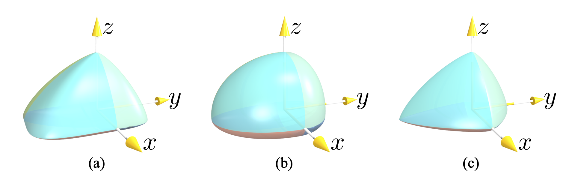 Poly-superellipsoids with
$r_x^+=1.0, r_x^-=0.5, r_y^+=0.8, r_y^- = 0.9, r_z^+ = 0.4, r_z^- = 0.6$
and (a) $\epsilon_1=0.4, \epsilon_2=1.5$, (b)
$\epsilon_1=\epsilon_2=1.0$, (c)
$\epsilon_1=\epsilon_2=1.5$.
Poly-superellipsoids with
$r_x^+=1.0, r_x^-=0.5, r_y^+=0.8, r_y^- = 0.9, r_z^+ = 0.4, r_z^- = 0.6$
and (a) $\epsilon_1=0.4, \epsilon_2=1.5$, (b)
$\epsilon_1=\epsilon_2=1.0$, (c)
$\epsilon_1=\epsilon_2=1.5$.
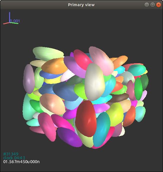
Here we give an exemplified script for packing of poly-superellipsoids as follows:
|
|
After running the script above, the user is expected to see a packing as shown in Fig. 3.19{reference-type=“ref” reference=“figpolysuperpacking”}.
 {#figpolysuperpacking
width=“10cm”}
{#figpolysuperpacking
width=“10cm”}
2.6 - Example 5: packing of superellipses
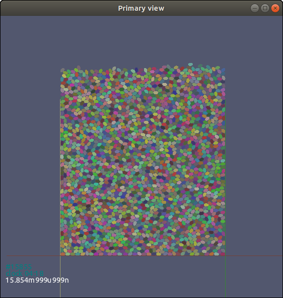
The surface function of a superellipse in the local Cartesian coordinates can be defined as $$\big|\frac{x}{r_x}\big|^{\frac{2}{\epsilon}} + \big|\frac{y}{r_y}\big|^{\frac{2}{\epsilon}} = 1$$ where $r_x$ and $r_y$ are referred to as the semi-major axis lengths in the direction of x, and y axies, respectively; and $\epsilon \in (0, 2)$ is the shape parameters determining the sharpness of particle edges or squareness of particle surface. Here we simulate packing of superellipses under gravity with the following script:
|
|
After running the above script with sudodem2d, the user can get a packing as shown in Fig. 3.20{reference-type=“ref” reference=“figpackingellipse”}.
 {#figpackingellipse width=“10cm”}
3 - Post-processing
Data
It is preferable to save a series of states during a simulation, i.e., periodically saving data using a PyRunner:
|
|
The Python module utilspost provides plentiful examples of post-processing, including some basic functions of stress-force-fabric computation and other pre-processing functions for visualization (e.g., writing vtk files of particles and 3D histograms of fabric). Based on this module, users can copy and modify for a self purpose or just call the module functions in a post-processing script, e.g.,
|
|
The Python module _superquadrics_utils also provides some auxiliary functions, e.g.,
-
outputParticles(filename) : filename, the file name for writing; output info of each particle, i.e., shape parameters $r_x$, $r_y$, $r_z$, $\epsilon_1$, $\epsilon_2$, position $x$, $y$, $z$, and orientation $q0$,$q1$,$q2$,$q3$ (equivalent to $q_w$, $q_x$, $q_y$, $q_z$ line by line. respectively).
-
outputParticlesbyIds(filename, ids) : filename, the file name for writing; ids, a list of ids for particles needed outputting; output info of each particle in the list ids, i.e., shape parameters $r_x$, $r_y$, $r_z$, $\epsilon_1$, $\epsilon_2$, position $x$, $y$, $z$, and orientation $q0$,$q1$,$q2$,$q3$ (equivalent to $q_w$, $q_x$, $q_y$, $q_z$ line by line. respectively).
-
outputWalls(filename) : filename, the file name for writing; output positions of all walls.
-
outputPOV(filename) : filename, the file name for writing; output a POV-Ray file of particles for render using POV-Ray.
-
outputVTK(filename,slices) : filename, the file name for writing; slices, number of slices a particle needed slicing in longitude; output a vtk file of particles for render using Paraview.
Scene Visualization
SudoDEM3D
For visualization, two free, open-source post-processing softwares, Paraview[^6] and POV-Ray[^7], are strongly recommended.
 {#figparaview width=“10cm”}
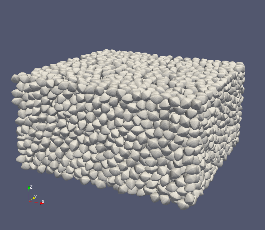
It is preferable to reproduce a high-resolution figure of particle configuration using post-processing softwares instead of a screenshot. As a demonstration, we load a state file named "shearend.xml.bz2" and output a vtk file or a pov file for post visualization.
|
|
Open Paraview, then import the vtk file "shearend.vtk" and click the button "Apply", so that the configuration of particles is visualized as shown in Fig. 4.2{reference-type=“ref” reference=“figshearendvtk”}. It is noteworthy that the function outputVTK processes a particle surface as a combination of many (determined by the argument slices, i.e., 15 herein) polygons, which would yield a large file (around 180 Mb in the presented example). The users may find ways to reduce the vtk file for a faster visualization in Paraview. One possible way is to show only the particles exposed in the view. Another possible way is to use the interface of built-in Superquadric source in Paraview.
 {#figshearendvtk width=“8cm”}
Another alternative approach is rendering the scene utilizing POV-Ray.
|
|
The users might revise the parameters of the camera in the POV file, i.e., "shearend.pov" here,
|
|
Light sources should be slightly adjusted as well.
|
|
In a terminal, run the following command to render the scene:
povray shearend.pov
For a high-resolution render, additional arguments are appended to the command,
povray shearend.pov +A0.01 +W1600 +H1200
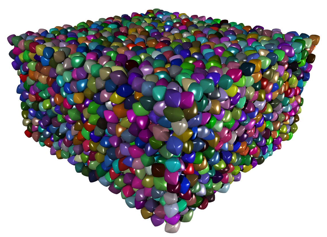
Image processing softwares, e.g., GIMP [^8], can be used to change image size or make a gif animation, etc. Fig. 4.3{reference-type=“ref” reference=“figshearend”} shows configuration of particles rendered by POV-Ray and cropped using GIMP.
 {#figshearend width=“8cm”}
The module snapshot provides functions for visualizing poly-superellipsoids. As an example, we load the state of final packing, and import the module and call the outPov function as follows:
|
|
we then get two files packingpolysuper.inc and packingpolysuper.pov. The first file packingpolysuper.inc includes macros for the definition of poly-superellipsoid and the particle information such as shape parameters, positions and orientations, like this:
|
|
The users are not suggested to edit this file though. But the second file packingpolysuper.pov includes some editable parameters as introduced above, and looks like this:
|
|
Then render it in a fresh terminal by typing
povray packingpolysuper.pov +A0.01 +W1600 +H1200
you will get a nice figure with higher quality as Fig. 4.4{reference-type=“ref” reference=“figpolypov”}.
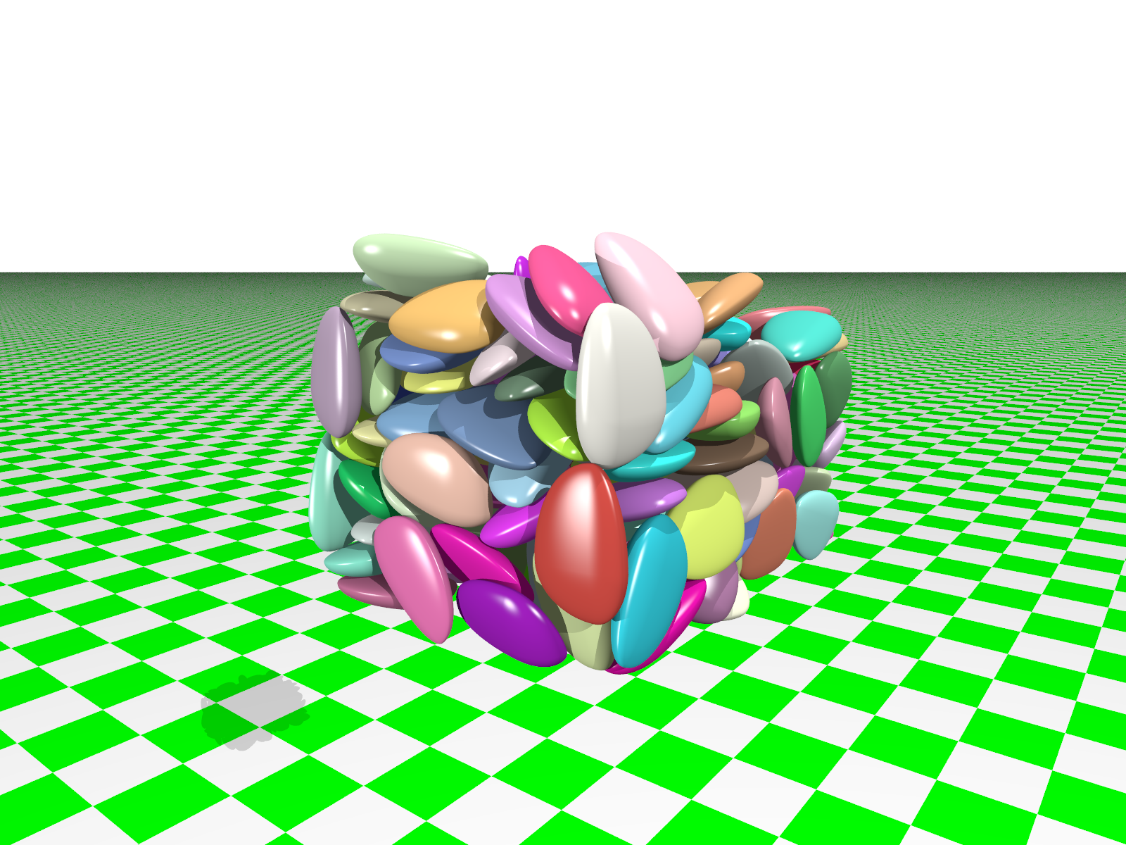 {#figpolypov width=“10cm”}
SudoDEM2D
Module _superellipse_utils provides a function drawSVG (see Sec. 5.2.2{reference-type=“ref” reference=“secmodsuperellipse”}) to dump the particle profiles and contact forces chains to a SVG file.
|
|
The output file test.svg is editable by using a text editor and/or Inkscape (recommended). Fig. 4.5{reference-type=“ref” reference=“figellipsesvg”} shows an exemplified snapshot of a packing of elliptic particles with periodic boundary conditions. Refer to the keywords of drawSVG for configuring the output figure.
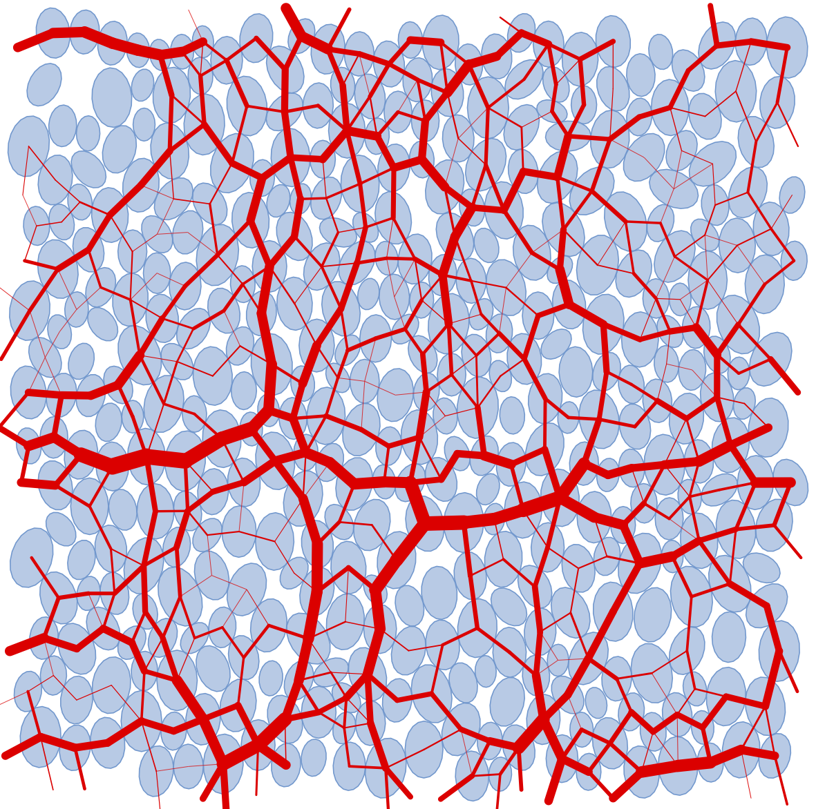 {#figellipsesvg width=“10cm”}
4 - Python Class Reference
SudoDEM3D
Basic classes
class State(inherits Serializable)
State of a body (spatial configuration, internal variables).
-
angMom(=Vector3r::Zero())
Current angular momentum -
angVel(=Vector3r::Zero())
Current angular velocity -
blockedDOFs
Degress of freedom where linear/angular velocity will be always constant (equal to zero, or to an user-defined value), regardless of applied force/torque. String that may contain ‘xyzXYZ’ (translations and rotations). -
dict() → dict
Return dictionary of attributes. -
inertia(=Vector3r::Zero())
Inertia of associated body, in local coordinate system. -
isDamped(=true)
Damping in Newtonintegrator can be deactivated for individual particles by setting this variable to FALSE. E.g. damping is inappropriate for particles in free flight under gravity but it might still be applicable to other particles in the same simulation. -
mass(=0)
Mass of this body -
ori
Current orientation. -
pos
Current position. -
refOri(=Quaternionr::Identity())
Reference orientation -
refPos(=Vector3r::Zero())
Reference position -
se3(=Se3r(Vector3r::Zero(), Quaternionr::Identity()))
Position and orientation as one object.
Module _superquadrics_utils
-
NewSuperquadrics2($r_x$, $r_y$, $r_z$, $\epsilon_1$, $\epsilon_2$, mat, rotate, isSphere)
Generate a Superquadric with isSphere option.-
$r_x$, $r_y$, $r_z$: float, semi-major axis lengths in x, y, and z axies.
-
$\epsilon_1$, $\epsilon_2$: float, shape parameters.
-
mat: Material, a material attached to the particle.
-
rotate: bool, with a random orientation or not.
-
isSphere: bool, particle is spherical or not.
-
-
NewSuperquadrics_rot2($r_x$, $r_y$, $r_z$, $\epsilon_1$, $\epsilon_2$, mat, $q_w$, $q_x$, $q_y$, $q_z$, isSphere)
Generate a Super-ellipsoid with specified quaternion components: $q_w$, $q_x$, $q_y$, $q_z$ with isSphere option.-
$r_x$, $r_y$, $r_z$: float, semi-major axis lengths in x, y, and z axies.
-
$\epsilon_1$, $\epsilon_2$: float, shape parameters.
-
mat: Material, a material attached to the particle.
-
isSphere: bool, particle is spherical or not.
-
$q_w$, $q_x$, $q_y$, $q_z$: float, components of a quaternion ($q_w$, $q_x$, $q_y$, $q_z$) representing the orientation of a particle.
-
-
outputWalls(filename)
Output positions of all walls in the scene.- filename: string, the name (with path) of the output file.
-
getSurfArea(id, w, h)
Get the surface area of a super-ellipsoid by a given particle id with resolution w and h (e.g., w=10,h=10). Larger w and h will yield more accurate results.-
id: int, the id of the given particle.
-
w, h: int, w$\times$h slices the particle surface will be discretized into.
-
-
outputParticles(filename)
Output information including id, shape parameters, position and orientation of all particles into a file.- filename: string, the name (with path) of the output file.
-
outputParticlesbyIds(filename, ids)
Output particles by a list of ids, referring to the last function. [Only for superellipsoids]-
filename: string, the name (with path) of the output file.
-
ids: list of int, a list of particle ids, e.g., [10, 24, 22].
-
-
NewPolySuperellipsoid(eps, rxyz, mat, rotate, isSphere, inertiaScale = 1.0)
Generate a PolySuperellipsoid.-
$eps$: Vector2, shape parameters, i.e., [$\epsilon_1$, $\epsilon_2$].
-
$rxyz$: Vector6, semi-major axis lengths in x, y, and z axies, i.e.,[$r_x^-$, $r_x^+$, $r_y^-$, $r_y^+$, $r_z^-$, $r_z^+$].
-
mat: Material, a material attached to the particle.
-
rotate: bool, with a random orientation or not.
-
isSphere: bool, particle is spherical or not.
-
inertialScale: float, scale the moment of inertia only. Do not set it if you are not sure the side effect.
-
-
NewPolySuperellipsoid_rot(eps, rxyz, mat, $q_w$, $q_x$, $q_y$, $q_z$, isSphere, inertiaScale = 1.0)
Generate a PolySuperellipsoid with specified quaternion components: $q_w$, $q_x$, $q_y$ and $q_z$.-
$eps$: Vector2, shape parameters, i.e., [$\epsilon_1$, $\epsilon_2$].
-
$rxyz$: Vector6, semi-major axis lengths in x, y, and z axies, i.e.,[$r_x^-$, $r_x^+$, $r_y^-$, $r_y^+$, $r_z^-$, $r_z^+$].
-
mat: Material, a material attached to the particle.
-
isSphere: bool, particle is spherical or not.
-
$q_w$, $q_x$, $q_y$ and $q_z$: float, components of a quaternion ($q_w$, $q_x$, $q_y$, $q_z$) representing the orientation of a particle.
-
inertialScale: float, scale the moment of inertia only. Do not set it if you are not sure the side effect.
-
-
outputPOV(filename)
Output Superellipsoids (including spheres) into a POV file for post-processing using POV-ray. [Only for superellipsoids and spheres]- filename: string, the name (with path) of the output file.
-
PolySuperellipsoidPOV(filename, ids = [], scale = 1.0)
Output PolySuperellipsoids into a POV file for post-processing using POV-ray. This function only output the particles' information to a POV file like *.inc, and the user may need to add some other info such as camera etc. See the module snapshot.-
filename: string, the name (with path) of the output file.
-
ids: list of int, a list of particle ids. A NULL list will output all particles by default.
-
scale: float, scale the length unit.
-
-
outputVTK(filename, slices)
Output Superellpisoids into a VTK file for post-processing using Paraview. [Only for superellipsoids]-
filename: string, the name (with path) of the output file.
-
slices: int, into how many slices the particle surface will be discretized.
-
Module _gjkparticle_utils
-
GJKSphere(radius,margin,mat)
-
radius, float, radius of the sphere.
-
margin, float, a small margin added to the surface for assisting contact detection.
-
mat, Material, a specified material attached to the particle.
-
-
GJKPolyhedron(vertices,extent,margin,mat, rotate)
-
vertices, a list of vertices, and each vertex is a list, e.g., $[x, y, z]$ for coordinates.
-
extent, a list of three components to scale the x, y, z dimensions; valid only if vertices has no elements (i.e., $ $); a randomly shaped polyhedron will be generated based on Voronoi tessellation.
-
margin, float, a small margin added to the surface for assisting contact detection.
-
mat, Material, a specified material attached to the particle.
-
rotate, bool, with random orientation or not.
-
-
GJKCone(radius, height, margin, mat, rotate)
-
radius, float, base radius of the cone.
-
height, float, height of the cone.
-
margin, float, a small margin added to the surface for assisting contact detection.
-
mat, Material, a specified material attached to the particle.
-
rotate, bool, with random orientation or not.
-
-
GJKCylinder(radius, height, margin, mat, rotate)
-
radius, float, radius of the cylinder.
-
height, float, height of the cylinder.
-
margin, float, a small margin added to the surface for assisting contact detection.
-
mat, Material, a specified material attached to the particle.
-
rotate, bool, with random orientation or not.
-
-
GJKCuboid(extent, margin,mat, rotate)
-
extent, a list of three floats, extent of the cuboid in the x, y, z dimensions.
-
margin, float, a small margin added to the surface for assisting contact detection.
-
mat, Material, a specified material attached to the particle.
-
rotate, bool, with random orientation or not.
-
Note: a margin is used to expand a particle for achieving a better computational efficiency, which however should be large enough for ensuring that collision occurs in this small region but small enough for shape fidelity.
Module snapshot
-
outputBoxPov(filename, x, y, z, r=0.001, wallMask=[1,0,1,0,0,1])
Output *.POV of a cubic box (x=[x_min, x_max], y=[y_min, y_max], z=[z_min, z_max]) for post-processing in Pov-ray.-
filename: string, the name (with path) of the output file.
-
x, y, z: Vector2, ranges of the cubic box along the three (x, y, z) directions.
-
r: float, thickness of the box edge.
-
wallMask, list of 6 int, corresponding to the six walls at (x-, x+, y-, y+, z-, z+). 1 to show and 0 to hide the wall.
-
-
outPov(fname,transmit=0,phong=1.0,singleColor=True,ids=[],scale=1.0, withbox = True)\
-
filename, string, the name (with path) of the output file.
-
transmit, float, parameter for transparency of particles, ranging between 0 and 1.
-
phong, float, parameter for highlighting the surface, ranging between 0 and 1.
-
singleColor, bool, whether to use a single color for all particles. If not, particles' colors would be the values defined in Shape.
-
ids, list of int, a list of particle ids that will be output. If no item are given, then all particles will be output by default.
-
scale, float, scale the unit.
The user is referred to POV-Ray’s Doc for more details on the two parameters (transmit and phong) and others that will be written to the output file by this function.
-
SudoDEM2D
Basic classes
Class State
State of a body (spatial configuration, internal variables).
-
angMom(=Vector2r::Zero())
Current angular momentum -
angVel(=Vector2r::Zero())
Current angular velocity -
blockedDOFs
Degress of freedom where linear/angular velocity will be always constant (equal to zero, or to an user-defined value), regardless of applied force/torque. String that may contain ‘xyZ’ (translations and rotations). -
dict() → dict
Return dictionary of attributes. -
inertia(=Vector2r::Zero())
Inertia of associated body, in local coordinate system. -
isDamped(=true)
Damping in Newtonintegrator can be deactivated for individual particles by setting this variable to FALSE. E.g. damping is inappropriate for particles in free flight under gravity but it might still be applicable to other particles in the same simulation. -
mass(=0)
Mass of this body -
ori
Current orientation. The orientation and rotation of a particle is represented by a Rotation2d object (see Rotation2D in the Eigen library), which has the following members and functions.
Class Rotation2d-
angle: float, rotation represented by an angle in rad.
-
toRotationMatrix(): Matrix2r, returns an equivalent 2x2 rotation matrix.
-
Identity(): Roation2d, returns an identity rotation.
-
smallestAngle(): float, returns the rotation angle in $[-\pi,\pi]$
-
inverse(): Roation2d, returns the inverse rotation
-
smallestPositiveAngle(): float, returns the rotation angle in $[0,2\pi]$
-
-
pos
Current position. -
refOri(=Rotation2D::Identity())
Reference orientation -
refPos(=Vector2r::Zero())
Reference position -
se2(=Se2r(Vector2r::Zero(), Rotation2d::Identity()))
Position and orientation as one object. -
vel(=Vector2r::Zero()) Current linear velocity.
Module _superellipse_utils
-
NewSuperellipse(rx, ry, epsilon, material, rotate, isSphere, z_dim =1.0)
Create a Superellipse
-
rx, ry: float, semi-axis length of the particle
-
epsilon: float, shape parameter of a superellipse
-
material: Material instance
-
rotate: bool, rotate the particle with random orientation?
-
isSphere: bool, is the superellipse a disk? A disk will speed up the computation.
-
z_dim: float, the virtual length at the z dimension, and set to 1.0 by default.
-
-
NewSuperellipse_rot(x, y, epsilon, material, miniAngle, isSphere, z_dim = 1.0)
Create a superellipse with certain orientation
-
rx, ry: float, semi-axis length of the particle
-
epsilon: float, shape parameter of a superellipse
-
material: Material instance
-
miniAngle: orientation of the particle specified by the angle between its rx-axis and the global x axis
-
isSphere: bool, is the superellipse a disk? A disk will speed up the computation.
-
z_dim: float, the virtual length at the z dimension, and set to 1.0 by default.
-
-
outputParticles(filename)
output particle info(rx,ry,eps,x,y,rotation angle) to a text file
-
drawSVG(filename, width_cm = 10.0, slice = 20, line_width = 0.1, fill_opacity = 0.5, draw_filled = true, draw_lines = true, color_po = false, po_color = Vector3r(1.0,0.0,0.0), solo_color = Vector3r(0,0,0), force_line_width = 0.001, force_fill_opacity = 0, force_line_color = Vector3r(1.0,1.0,1.0), draw_forcechain = false)
Output particle profiles and contact force chains into a SVG file.
-
filename: string, the name of the output file
-
width_cm: float, width (in centimeters) in the SVG header
-
slice: int, to how many slices a Superellipse will be discretized
-
line_width: float, the line width of the edge of a Superellipse
-
fill_opacity: float, the opacity of the fill color in a Superellipse
-
draw_filled: bool, wheter to fill a Superellipse with a color
-
draw_lines: bool, whether to draw the out profile of a Superellipse
-
color_po: bool, whether to use a fill color to identify the orientation of a Superellipse
-
po_color: Vector3r, the fill color to identify the orientation of a Superellipse
-
solo_color: Vector3r, a solor color to fill a Superellipse. If its norm is zero, then use the color defined by po_color or shape$\rightarrow$color
-
force_line_width: float, the line width of the force chain with the average normal contact force
-
force_fill_opacity: float, the opacity of force chains
-
force_line_color: Vector3r, the color of the force chain
-
draw_forcechain: bool, whether to draw the contact force chain that will be superposed with the particles
-
Module _utils
-
unbalancedForce(useMaxForce=false)
Compute the ratio of mean (or maximum, if *useMaxForce*) summary force on bodies and mean force magnitude on interactions. For perfectly static equilibrium, summary force on all bodies is zero (since forces from interactions cancel out and induce no acceleration of particles); this ratio will tend to zero as simulation stabilizes, though zero is never reached because of finite precision computation. Sufficiently small value can be e.g. 1e-2 or smaller, depending on how much equilibrium it should be.
-
getParticleVolume2D()
Compute the total volume (area for 2D) of particles in the scene. -
getMeanCN()
Get the mean coordination number of a packing -
changeParticleSize2D(alpha)
expand a particle by a given coefficient -
getVoidRatio2D(cellArea=1)
Compute 2D void ratio. Keyword cellArea is effective only for aperioidc cell -
getStress2D(z_dim=1)
Compute overall stress of periodic cell -
getFabricTensorCN2D()
Fabric tensor of contact normal -
getFabricTensorPO2D()
Fabric tensor of particle orientation along the rx axis -
getStressAndTangent2D(z_dim=1,symmetry=true)
Compute overall stress of periodic cell using the same equation as function getStress. In addition, the tangent operator is calculated using the equation: $S_{ijkl}=\frac{1}{V}\sum_{c}(k_n n_i l_j n_k l_l + k_t t_i l_j t_k l_l)$ float volume: same as in function getStress bool symmetry: make the tensors symmetric.
return: macroscopic stress tensor and tangent operator as py::tuple -
getStressTangentThermal2D(z_dim=1, symmetry =true)
Compute overall stress of periodic cell using the same equation as function getStress. In addition, the tangent operator is calculated using the equation: $S_{ijkl}=\frac{1}{V}\sum_{c}(k_n n_i l_j n_k l_l + k_t t_i l_j t_k l_l)$ float volume: same as in function getStress bool symmetry: make the tensors symmetric. Finally, the thermal conductivity tensor is calculated based on the formular in PFC. macroscopic stress tensor and tangent operator as py::tuple
Module utils
-
disk(center, radius, z_dim=1, dynamic=None, fixed=False, wire=False, color=None, highlight=False, material=-1,mask=1)
Create a disk with given parameters; mass and inertia computed automatically.-
center: Vector2, center
-
radius: float, radius
-
dynamic: float, deprecated, see "fixed"
-
fixed: float, generate the body with all DOFs blocked?
-
material: specify ‘Body.material’; different types are accepted:
-
int: O.materials[material] will be used; as a special case, if material==-1 and there is no shared materials defined, utils.defaultMaterial() will be assigned to O.materials[0]
-
string: label of an existing material that will be used
-
‘Material’ instance: this instance will be used
-
callable: will be called without arguments; returned Material value will be used (Material factory object, if you like)
-
-
int mask: ‘Body.mask’ for the body
-
wire: display as wire disk?
-
highlight: highlight this body in the viewer?
-
Vector2-or-None: body’s color, as normalized RGB; random color will be assigned if “None”.
-
-
wall(position, axis, sense=0, color=None, material=-1, mask=1)
Return ready-made wall body.-
position: float-or-Vector3 , center of the wall. If float, it is the position along given axis, the other 2 components being zero
-
axis: {0,1} , orientation of the wall normal (0,1) for x,y
-
sense: {-1,0,1} , sense in which to interact (0: both, -1: negative, +1: positive; see ‘Wall’)
See ‘utils.disk'’s documentation for meaning of other parameters.
-
-
fwall(vertex1, vertex2, dynamic=None, fixed=True, color=None, highlight=False, noBound=False, material=-1, mask=1, chain=-1)
Create fwall with given parameters.-
vertex1: Vector2, coordinates of vertex1 in the global coordinate system.
-
vertex2: Vector2, coordinates of vertex2 in the global coordinate system.
-
noBound: bool, set ‘Body.bounded’
-
color: Vector3-or-None , color of the facet; random color will be assigned if ‘None’.
See ‘utils.disk'’s documentation for meaning of other parameters.
-