We prepared several examples to show a quick start of using SudoDEM,
and the corresponding script for each example is available on the
website or the Github repository
(https://github.com/SwaySZ/ExamplesSudoDEM).
1 - Example 0: run a simulation
Here’s where your user finds out if your project is for them.
This example will show the ingredients of a simulation by simulating a
sphere free falling onto a ground. We prepare a Python script named
‘example0.py’ at our work directory (e.g., /home/xxx/example'). Open a
terminal, and type ‘sudodem3d example0.py’ if the work directory is at
‘/home/xxx/example/’ otherwise providing a relative or absolute path of
‘example0.py’.
# A sphere free falling on a ground under gravityfromsudodemimportutils# module utils has some auxiliary functions#1. we define materials for particlesmat=RolFrictMat(label="mat1",Kn=1e8,Ks=7e7,frictionAngle=math.atan(0.0),density=2650)# material 1 for particleswallmat1=RolFrictMat(label="wallmat1",Kn=1e8,Ks=0,frictionAngle=0.)# material 2 for walls# we add the materials to the container for materials in the simulation.# O can be regarded as an object for the whole simulation.# We can see that materials is a property of O, so we use a dot operation (O.materials) to get the property (materials).O.materials.append(mat)# materials is a list, i.e., a container for all materials involving in the simulationsO.materials.append(wallmat1)# adding a material to the container (materials) so that we can easily access it by its label. See the definition of a wall below.#create a spherical particlesp=sphere((0,0,10.0),1.0,material=mat)O.bodies.append(sp)# create the ground as an infinite plane wallground=utils.wall(0,axis=2,sense=1,material='wallmat1')# utils.wall defines a wall with normal parallel to one axis of the global Cartesian coordinate system. The first argument (here = 0) specifies the location of the wall, and with the keyword axis (here = 2, axis has a value of 0, 1, 2 for x, y, z axies respectively) we know that the normal of the wall is along z axis with centering at z = 0 (0, specified by the first argument); the second keyword sense (here = 1, sense can be -1, 0, 1 for negative, both, and positive sides respectively) specifies that the positive side (i.e., the normal points to the positive direction of the axis) of the wall is activated, at which we will compute the interaction of a particle and this wall; the last keyword materials specifies a material to this wall, and we assign a string (i.e., the label of wallmat1) to the keyword, and directly assigning the object of the material (i.e., wallmat1 returned by RolFrictMat) is also acceptable.O.bodies.append(ground)# add the ground to the body container# define a function invoked periodically by a PyRunnerdefrecord_data():#open a filefout=open('data.dat','a')#create/open a file named 'data.dat' in append mode#we want to record the position of the spherep=O.bodies[0]# the sphere has been appended into the list O.bodies, and we can use the corresponding index to access it. We have added two bodies in total to O.bodies, and the sphere is the first one, i.e., the index is 0.# p is the object of the sphere# as a body object, p has several properties, e.g., state, material, which can be listed by p.dict() in the commandline.pos=p.state.pos# get the position of the sphereprint>>fout,O.iter,pos[0],pos[1],pos[2]# we print the iteration number and the position (x,y,z) into the file fout.# then, close the file and release resourcefout.close()# create a Newton engine by which the particles move under Newton's Lawnewton=NewtonIntegrator(damping=0.1,gravity=(0.,0.0,-9.8),label="newton")# we set a local damping of 0.1 and gravitational acceleration -9.8 m/s2 along z axis.# the engine container is the kernel part of a simulation# During each time step, each engine will run one by one for completing a DEM cycle.O.engines=[ForceResetter(),# first, we need to reset the force container to store upcoming contact forces# next, we conduct the broad phase of contact detection by comparing axis-aligned bounding boxs (AABBs) to rule out those pairs that are definitely not contacting.InsertionSortCollider([Bo1_Sphere_Aabb(),Bo1_Wall_Aabb()],verletDist=0.2*0.01),# then, we execute the narrow phase of contact detectionInteractionLoop(# we will loop all potentially contacting pairs of particles[Ig2_Sphere_Sphere_ScGeom(),Ig2_Wall_Sphere_ScGeom()],# for different particle shapes, we will call the corresponding functions to compute the contact geometry, for example, Ig2_Sphere_Sphere_ScGeom() is used to compute the contact geometry of a sphere-sphere pair.[Ip2_RolFrictMat_RolFrictMat_RolFrictPhys()],# we will compute the physical properties of contact, e.g., contact stiffness and coefficient of friction, according to the physical properties of contacting particles.[RollingResistanceLaw(use_rolling_resistance=False)]# Next, we compute contact forces in terms of the contact law with the info (contact geometric and physical properties) computed at last two steps.),newton,# finally, we compute acceleration and velocity of each particle and update their positions.#at each time step, we have a PyRunner function help to hack into a DEM cycle and do whatever you want, e.g., changing particles' states, and saving some data, or just stopping the program after a certain running time. PyRunner(command='record_data()',iterPeriod=10000,label='record',dead=False)]# we need to set a time stepO.dt=1e-5# clean the file data.dat and write a file headfout=open('data.dat','w')# we open the file in a write mode so that the file will be cleanprint>>fout,'iter, x, y, z'# write a file headfout.close()# close the file# run the simulation# you have two choices:# 1. give a command here, like,# O.run()# you can set how many iterations to runO.run(1600000)# 2. clike the run button at the GUI controler
Run the simulation by typing the following command in a terminal:
We can take a quick view on the recorded data using gnuplot. Install
gnuplot by typing the following command in a terminal:
sudo apt install gnuplot
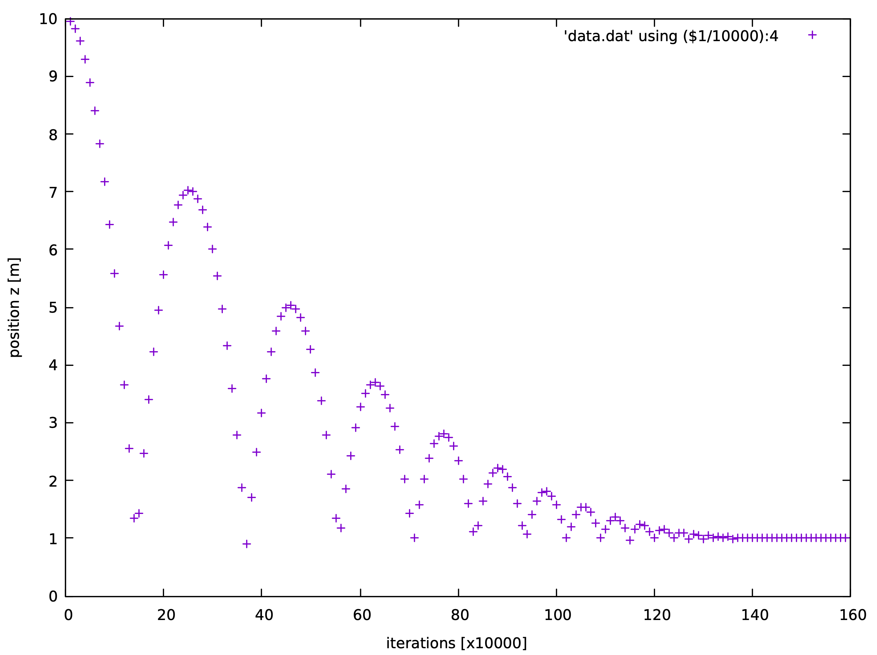
Then, open gnuplot and plot the data as shown in Fig.
3.1{reference-type=“ref” reference=“figsinglesp”}:
$> gnuplot
    gnuplot> plot 'data.dat' using ($1/10000):4; set xlabel 'iterations [x10000]'; set ylabel 'position z [m]'
The z-position of a sphere free falling onto a ground.
2 - Example 1: packing of super-ellipsoids
Here’s where your user finds out if your project is for them.
The surface function of a superellipsoid in the local Cartesian
coordinates can be defined as $$\label{eqsurface}
\Big(\big|\frac{x}{r_x}\big|^{\frac{2}{\epsilon_1}} + \big|\frac{y}{r_y}\big|^{\frac{2}{\epsilon_1}}\Big)^{\frac{\epsilon_1}{\epsilon_2}} + \big|\frac{z}{r_z}\big|^{\frac{2}{\epsilon_2}} = 1$$
where $r_x, r_y$ and $r_z$ are referred to as the semi-major axis
lengths in the direction of x, y, and z axies, respectively; and
$\epsilon_i (i=1,2)$ are the shape parameters determining the sharpness
of particle edges or squareness of particle surface. Varying
$\epsilon_i$ between 0 and 2 yields a wide range of convex-shaped
superellipsoid. Two functions for generating a superellipsoid are
highlighted below (see Sec.
5.1.2{reference-type=“ref”
reference=“modsuperquadrics”}):
################################################ granular packing of super-ellipsoids# We position particles at a lattice grid, # then particles free fall into a cubic box.################################################ import some modulesfromsudodemimport_superquadrics_utilsfromsudodem._superquadrics_utilsimport*importmathimportrandomasrandimportnumpyasnp########define some parameters#################isSphere=Falsenum_x=5num_y=5num_z=20R=0.1#######define some auxiliary functions##########define a latice grid#R: distance between two neighboring nodes#num_x: number of nodes along x axis#num_y: number of nodes along y axis#num_z: number of nodes along z axis#return a list of the postions of all nodesdefGridInitial(R,num_x=10,num_y=10,num_z=20):pos=list()foriinrange(num_x):forjinrange(num_y):forkinrange(num_z):x=i*R*2.0y=j*R*2.0z=k*R*2.0pos.append([x,y,z])returnpos#generate a sampledefGenSample(r,pos):forpinpos:epsilon1=rand.uniform(0.7,1.6)epsilon2=rand.uniform(0.7,1.6)a=rb=r*rand.uniform(0.4,0.9)#aspect ratioc=r*rand.uniform(0.4,0.9)body=NewSuperquadrics2(a,b,c,epsilon1,epsilon2,p_mat,True,isSphere)body.state.pos=pO.bodies.append(body)#########setup a simulation##################### material for particlesp_mat=SuperquadricsMat(label="mat1",Kn=1e5,Ks=7e4,frictionAngle=math.atan(0.3),density=2650,betan=0,betas=0)# betan and betas are coefficients of viscous damping at contact, no viscous damping with 0 by default.# material for the side wallswall_mat=SuperquadricsMat(label="wallmat",Kn=1e6,Ks=7e5,frictionAngle=0.0,betan=0,betas=0)# material for the bottom wallwallmat_b=SuperquadricsMat(label="wallmat",Kn=1e6,Ks=7e5,frictionAngle=math.atan(1),betan=0,betas=0)# add materials to O.materialsO.materials.append(p_mat)O.materials.append(wall_mat)O.materials.append(wallmat_b)# create the box and add it to O.bodiesO.bodies.append(utils.wall(-R,axis=0,sense=1,material=wall_mat))#left wall along x axisO.bodies.append(utils.wall(2.0*R*num_x-R,axis=0,sense=-1,material=wall_mat))#right wall along x axisO.bodies.append(utils.wall(-R,axis=1,sense=1,material=wall_mat))#front wall along y axisO.bodies.append(utils.wall(2.0*R*num_y-R,axis=1,sense=-1,material=wall_mat))#back wall along y axisO.bodies.append(utils.wall(-R,axis=2,sense=1,material=wallmat_b))#bottom wall along z axis# create a lattice gridpos=GridInitial(R,num_x=num_x,num_y=num_y,num_z=num_z)# get positions of all nodes# create particles at each nodesGenSample(R,pos)# create engines# define a Newton enginenewton=NewtonIntegrator(damping=0.1,gravity=(0.,0.,-9.8),label="newton",isSuperquadrics=1)# isSuperquadrics: 1 for superquadricsO.engines=[ForceResetter(),InsertionSortCollider([Bo1_Superquadrics_Aabb(),Bo1_Wall_Aabb()],verletDist=0.2*0.1),InteractionLoop([Ig2_Wall_Superquadrics_SuperquadricsGeom(),Ig2_Superquadrics_Superquadrics_SuperquadricsGeom()],[Ip2_SuperquadricsMat_SuperquadricsMat_SuperquadricsPhys()],# collision "physics"[SuperquadricsLaw()]# contact law),newton]O.dt=5e-5
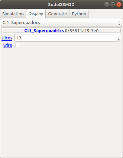
With a GUI controller, we can click ‘show 3D’ button at the panel
‘Simulation’ to display the simulating scene. On the ‘Display’ panel,
select the render ‘Gl1_Superquadrics’ to configure the resolution of
solid or wireframe particles, as shown in Fig.
3.3{reference-type=“ref” reference=“figguidisplay”}.
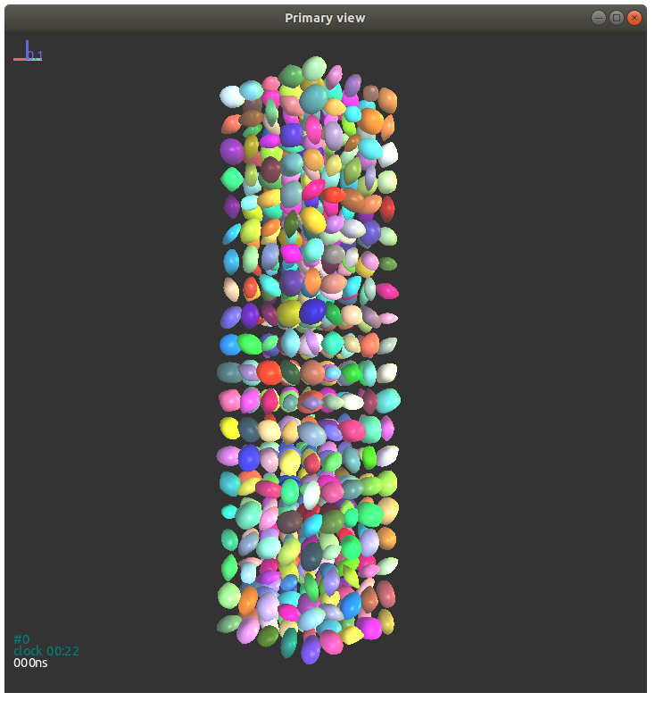
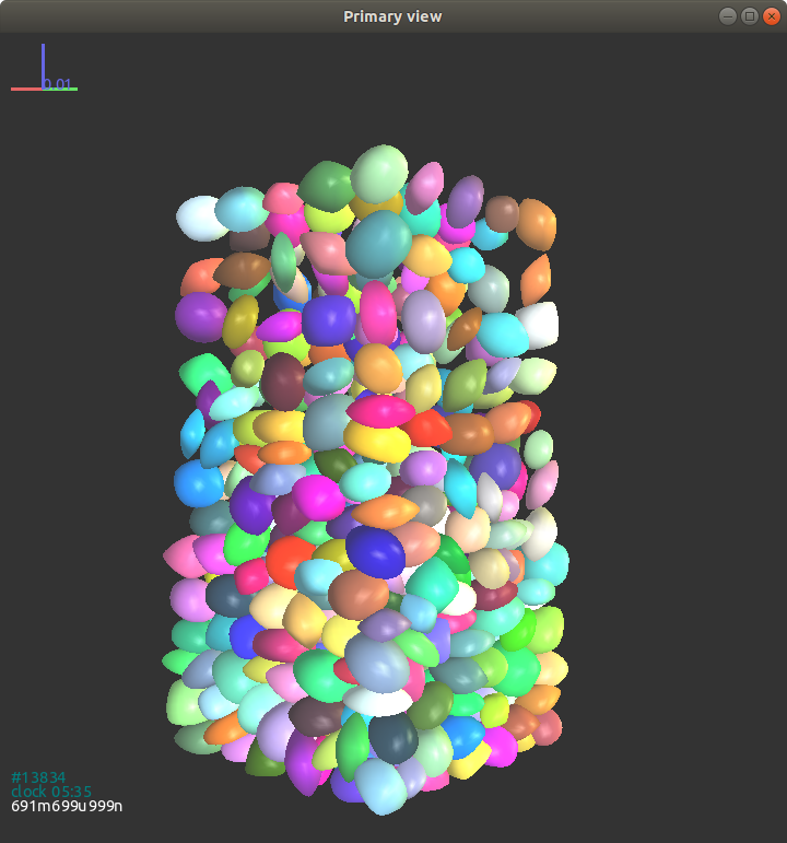
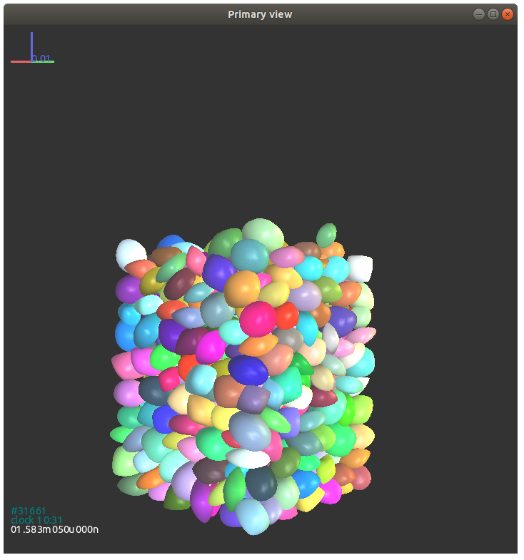
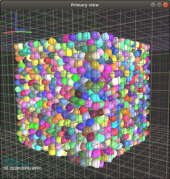
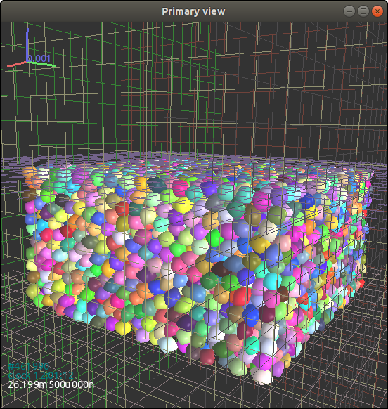
Figs. 3.4{reference-type=“ref” reference=“figexp11”} -
3.6{reference-type=“ref” reference=“figexp13”} show
simulations of packing of superellipsoids at different states for the
presented example.
Several properties and methods for a shape Superquadrics are listed
below:
Properties:
$r_x$, $r_y$, $r_z$: float, semi-major axis lengths in x, y, and
z axies.
geteps(): Vector2, return particle’s eps1 and eps2.
Here is an example to get the volume of a particle with an id of 100:
volume = O.bodies[100].shape.getVolume()
A general method to list all properties of an object is as follows:
O.bodies[100].dict()
The output is like follows:
{'bound': <Aabb instance at 0x56072ec83da0>,
 'chain': -1,
 'clumpId': -1,
 'flags': 3,
 'groupMask': 1,
 'id': 100,
 'iterBorn': 0,
 'material': <SuperquadricsMat instance at 0x56072e6ed5f0>,
 'shape': <Superquadrics instance at 0x56072ec83b60>,
 'state': <State instance at 0x56072ec839e0>,
 'timeBorn': 0.0}
We can see that the properties are printed in a dict form. Note that the
value enclosed by pointy brackets is another object (actually, instance
of an object with a specified memory address), which means that we can
further access it using the ".dict()" method. Again, the properties of
the object State can be accessed by:
Here we give an example to list ids and positions of all
superellipsoids:
for b in O.bodies: # loop all bodies in the simulation
    # we have to check if the present body is a superellipsoid or others, e.g., a wall
    if isinstance(b.shape, Superquadrics): # if it is a superellipsoid, then to do
        pid = b.id # get the id of particle b
        pos = b.state.pos # get the position of particle b
        print pid, pos
3 - Example 2: triaxial tests of super-ellipsoids
Here’s where your user finds out if your project is for them.
This example shows a triaxial compression simulation of superellipsoids
using an Engine CompressionEngine. The users can also customized their
engines or compression procedures easily via a PyRunner Engine. Here is
a basic setup of CompressionEngine for consolidation and compression
below.
Consolidation
 1
 2
 3
 4
 5
 6
 7
 8
 9
10
11
12
13
14
15
triax=CompressionEngine(goalx=1.0e5,# confining stress 100 kPagoaly=1.0e5,goalz=1.0e5,savedata_interval=10000,echo_interval=2000,continueFlag=False,max_vel=100.0,gain_alpha=0.5,f_threshold=0.01,#1-f/goalfmin_threshold=0.01,#the ratio of deviatoric stress to mean stressunbf_tol=0.01,#unblanced force ratiofile='record-con')
goalx = goaly = goalz = confining stress
savedata_interval: the interval of DEM iterations for saving
some data (Axial Strain, Volumetric Strain, Mean Stress and
DeviatorStress) into a file specified by file. Deprecated for
consolidation.
echo_interval: the interval of DEM iterations for outputting
information (Iterations, Unbalanced force ratio, stresses in x,
y, z directions) in the terminal
continueFlag: reserved keyword for continuing consolidation or
compression.
max_vel: the maximum velocity of a wall, which is useful to
constrain the movement of a wall during confining.
gain_alpha $\alpha$: guiding the movement of the confining
walls. $$v_w = \alpha \frac{f_w - f_g}{\Delta t \sum k_n}$$
where $v_w$ is the velocity of a confining wall at the next time
step; $f_w$ and $f_g$ are the present and goal confining forces,
respectively; $\Delta t$ is the time step, and $\sum k_n$ is the
summation of normal contact stiffness from all particle-wall
contacts on this wall.
f_threshold $\alpha_f$: a target ratio of the deviation of the
present stress from the goal to the goal, i.e.,
$$\alpha_f = \frac{|f_w-f_g|}{f_g}$$
fmin_threshold $\beta_f$: a target ratio of the deviatoric
stress $q$ to the mean stress $p$, i.e.,
$$\beta_f = \frac{q}{p},\quad p= \frac{\sigma_{ii}}{3},\quad q=\sqrt{\frac{3}{2}\sigma_{ij}^{'}\sigma_{ij}^{'}}$$
$$\sigma_{ij} = \frac{1}{V}\sum_{c\in V}f_i^cl_j^c,\quad \sigma_{ij}^{'}=\sigma_{ij}-p\delta_{ij}$$
where $\sigma_{ij}$ is the stress tensor with an assembly, and
$\sigma_{ij}^{'}$ is its corresponding deviatoric part; $V$ is
the total volume of the specimen; $f^c$ and $l^c$ are the
contact force and branch vector at contact $c$, respectively,
and $\delta_{ij}$ is the Kronecker delta.
unbf_tol $\gamma_f$: a target unbalanced force ratio defined
as
$$\gamma_f = \frac{\sum\limits_{B_i\in V} |\sum\limits_{j\in B_i}f^c_j+f^b_j|}{2\sum\limits_{c\in V}|f^c|}$$
Note: the consolidation ends up with that all $\alpha_f$,
$\beta_f$ and $\gamma_f$ reach the targets.
z_servo: a False value will trigger a strain (or displacement)
control in the z direction, and in this case goalz needs a
strain rate.
ramp_interval: iterations needed for reaching a constant
strain rate. This keyword is designed to mimic a continuing
loading at laboratory, but it seems not too valued and setting a
small value to kindly deprecate it.
ramp_chunks: number of intervals to reach the constant strain
rate combined with the keyword ramp_interval. It will be
deprecated as does ramp_interval.
target_strain: at this level of strain the shear procedures
ends. The strain is ogarithmic strain.
Note: to ensure quasi-static behavior during shear, the shear
strain rate should be sufficiently small. Specifically, the
inertial number $I$ should be maintained less than $10^{-3}$
$$I = \dot{\epsilon_1}\frac{\hat{d}}{\sqrt{\sigma_0/\rho}}$$
where $\dot{\epsilon_1}=\mathrm{d}\epsilon_1/\mathrm{d}t$ is the
major principal strain rate; $\hat{d}$ and $\rho$ are the
average diameter and material density of particles respectively;
$\sigma_0$ is the confining stress.
As a demonstration, we first give an example of consolidation as
follows:
##################################################fromsudodemimportplot,_superquadrics_utilsfromsudodem._superquadrics_utilsimport*importmathimportrandomasrandrand.seed(11245642)####################################################epsilon=1.4isSphere=Falseboxsize=[16.2e-3,16.2e-3,16.2e-3]#############################some auxiliary functions#generate a sample of monodisperse superellipsoids with random orientaions and positionsdefgen_sample(width,depth,height,r_max=1.0e-3):b_num_tot=5000forjinrange(b_num_tot):rb=r_max*0.5x=rand.uniform(rb,width-rb)y=rand.uniform(rb,depth-rb)z=rand.uniform(rb,height-rb)r=r_max*0.5b=NewSuperquadrics2(r*1.25,r,r,epsilon,epsilon,mat,True,isSphere)b.state.pos=(x,y,z)O.bodies.append(b)#Materials definitionmat=SuperquadricsMat(label="mat1",Kn=3e4,Ks=3e4,frictionAngle=math.atan(0.1),density=2650e4)#define Material with default valueswallmat1=SuperquadricsMat(label="wallmat1",Kn=1e6,Ks=0.,frictionAngle=0.)#define Material with default valueswallmat2=SuperquadricsMat(label="wallmat2",Kn=1e6,Ks=0.,frictionAngle=0.)#define Material with default valuesO.materials.append(mat)O.materials.append(wallmat1)O.materials.append(wallmat2)##################################################create confining walls############################################O.bodies.append(utils.wall(0,axis=0,sense=1,material='wallmat1'))#left xO.bodies.append(utils.wall(boxsize[0],axis=0,sense=-1,material='wallmat1'))#right xO.bodies.append(utils.wall(0,axis=1,sense=1,material='wallmat1'))#front yO.bodies.append(utils.wall(boxsize[1],axis=1,sense=-1,material='wallmat1'))#back yO.bodies.append(utils.wall(0,axis=2,sense=1,material='wallmat2'))#bottom zO.bodies.append(utils.wall(boxsize[2],axis=2,sense=-1,material='wallmat2'))#top z#####create particlesgen_sample(boxsize[0],boxsize[1],boxsize[2])####function for saving data (e.g., simulation states here)defsavedata():O.save(str(O.time)+'.xml.bz2')######################################### ####triax engine#CAUTION: the CompressionEngine regards the first six bodies as confining walls by default. So the walls should be generated first.triax=CompressionEngine(goalx=1.0e5,# confining stress 100 kPagoaly=1.0e5,goalz=1.0e5,savedata_interval=10000,echo_interval=2000,continueFlag=False,max_vel=10.0,gain_alpha=0.5,f_threshold=0.01,#1-f/goalfmin_threshold=0.01,#the ratio of deviatoric stress to mean stressunbf_tol=0.01,#unblanced force ratiofile='record-con',)############################newton=NewtonIntegrator(damping=0.3,gravity=(0.,0.,0.),label="newton",isSuperquadrics=1)O.engines=[ForceResetter(),InsertionSortCollider([Bo1_Superquadrics_Aabb(),Bo1_Wall_Aabb()],verletDist=0.1e-3),InteractionLoop([Ig2_Wall_Superquadrics_SuperquadricsGeom(),Ig2_Superquadrics_Superquadrics_SuperquadricsGeom()],[Ip2_SuperquadricsMat_SuperquadricsMat_SuperquadricsPhys()],[SuperquadricsLaw()]),triax,newton,PyRunner(command='quiet_ball()',iterPeriod=2,iterLast=50000,label='calm',dead=False),PyRunner(command='savedata()',realPeriod=7200.0,label='savedata',dead=False)#saving data every two hours]#delete the balls outside the boxdefdel_balls():num_del=0#wall positionleft=O.bodies[0].state.pos[0]#xright=O.bodies[1].state.pos[0]front=O.bodies[2].state.pos[1]#yback=O.bodies[3].state.pos[1]bottom=O.bodies[4].state.pos[2]#ztop=O.bodies[5].state.pos[2]forbinO.bodies:ifisinstance(b.shape,Superquadrics):(x,y,z)=b.state.posifx>rightorx<leftory<frontory>backorz<bottomorz>top:O.bodies.erase(b.id)num_del+=1printstr(num_del)+" particles are deleted!"defquiet_ball():globalcalm_numnewton.quiet_system_flag=Trueifcalm_num>2000:O.engines[-2].iterPeriod=5calm_num+=5else:calm_num+=2ifcalm_num>40000:ifcalm_num<40010:print"calm procedure is over"del_balls()ifcalm_num>50000:O.engines[-2].dead=TrueO.save("init_assembly.xml.bz2")#consolidation beginstriax.dead=Falseprint"consolidation begins"O.dt=1e-4triax.dead=Truecalm_num=0
The output in the terminal is akin to the follows:
calm procedure is over
0 particles are deleted!
consolidation begins
Iter 50000 Ubf 0.483161, Ss_x:9.67986e-05, Ss_y:4.15364e-05, Ss_z:6.1184e-05, e:0.992618
Iter 52000 Ubf 0.461741, Ss_x:1.2412, Ss_y:1.06812, Ss_z:1.10116, e:0.854445
Iter 54000 Ubf 0.263699, Ss_x:1.75334, Ss_y:1.98567, Ss_z:1.62181, e:0.757469
Iter 56000 Ubf 0.118329, Ss_x:3.06302, Ss_y:3.54818, Ss_z:3.22986, e:0.679106
Iter 58000 Ubf 0.0110747, Ss_x:22.0177, Ss_y:21.3303, Ss_z:21.3485, e:0.614824
Iter 60000 Ubf 0.000577066, Ss_x:91.4199, Ss_y:89.6039, Ss_z:89.1057, e:0.58984
Iter 62000 Ubf 0.000128293, Ss_x:100.012, Ss_y:99.7251, Ss_z:99.6123, e:0.587807
consolidation completed!
After consolidation (see the snapshot in Fig.
3.7{reference-type=“ref” reference=“figex2consol”}), we
obtain a state file by
1
O.save("final_con.xml.bz2")
Then, the consolidated assembly is subjected to triaxial compression
with the following scripts.
##################################################fromsudodemimportplot,_superquadrics_utilsfromsudodem._superquadrics_utilsimport*importmathsaving_num=0####################################################defsavedata():globalsaving_numsaving_num+=1#print "testing, no data saved"O.save('shear'+str(saving_num)+'.xml.bz2')defquiet_system():foriinO.bodies:i.state.vel=(0.,0.,0.)i.state.angVel=(0.,0.,0.)suffix=""O.load("final_con"+suffix+".xml.bz2")triax=O.engines[3]O.dt=5e-5friction=0.5O.materials[0].frictionAngle=math.atan(friction)if1:foritrinO.interactions:id=min(itr.id1,itr.id2)ifid>5:itr.phys.tangensOfFrictionAngle=friction#itr.phys.betan = 0.5##########################shear begins#########################defshear():quiet_system()triax.z_servo=Falsetriax.ramp_interval=10triax.ramp_chunks=2triax.file="sheardata"+suffixtriax.goalz=0.01triax.goalx=1e5triax.goaly=1e5triax.savedata_interval=2500triax.echo_interval=2000triax.target_strain=0.4shear()O.engines[-1].iterPeriod=2500O.engines[-1].realPeriod=0.0
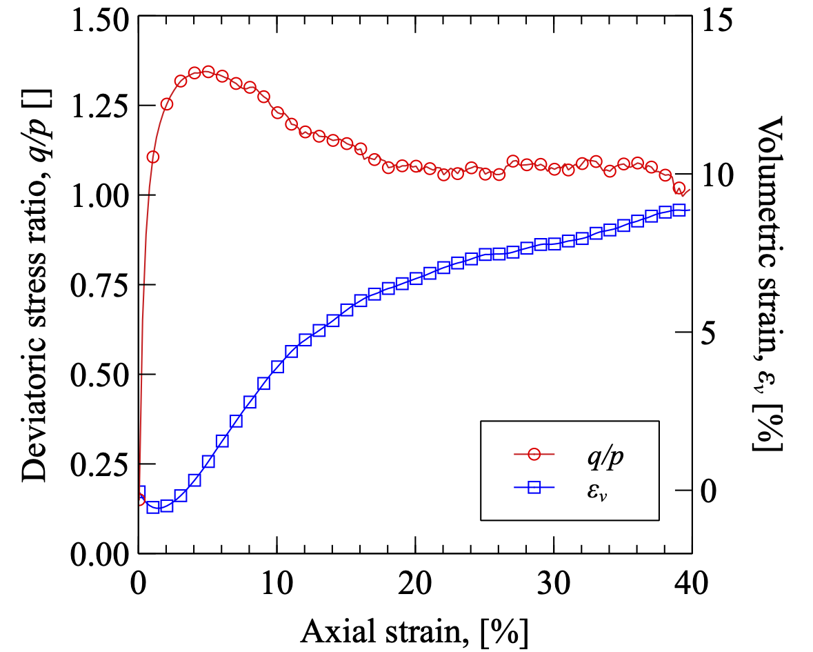
The compression ends up with an axial strain of 40%, and the final
configuration of particles is shown in Fig.
3.8{reference-type=“ref” reference=“figex2shear”}.
The macroscopic mechanical response of a granular material during
shearing can be quantified by the stress tensor that is calculated from
discrete measurements with the following definition:
$$\label{eqDEMstress}
\sigma_{ij} = \frac{1}{V} \sum_{c \in V} f_i^c l_j^c$$ where $V$ is the
total volume of the assembly, $f^c$ is the contact force at the contact
$c$, and $l^c$ is the branch vector joining the the centres of the two
contacting particles at contact $c$. The mean stress $p$ and the
deviatoric stress $q$ are defined as: $$p = \frac{1}{3}\sigma_{ii},\quad
q = \sqrt{\frac{3}{2} \sigma_{ij}^{'}\sigma_{ij}^{'}}$$ where
$\sigma_{ij}^{'}$ is the deviatoric part of stress tensor $\sigma_{ij}$.
Given that the cubical specimens are confined by rigid walls, the axial
strain $\epsilon_z$ and the volumetric strain $\epsilon_v$ can be
approximately calculated from the positions of the boundary walls, i.e.,
$$\epsilon_z = \int_{H_0}^{H}\frac{\mathrm{d}h}{h}=-\ln\frac{H_0}{H},\quad
\epsilon_v = \epsilon_x+\epsilon_y+\epsilon_z=\int_{V_0}^{V}\frac{\mathrm{d}v}{v}=-\ln\frac{V_0}{V}$$
where $H$ and $V$ are the height and volume of the specimen during
shearing, respectively, and $H_0$ and $V_0$ are their initial values
before shear. Positive values of volumetric strain represent dilatancy.
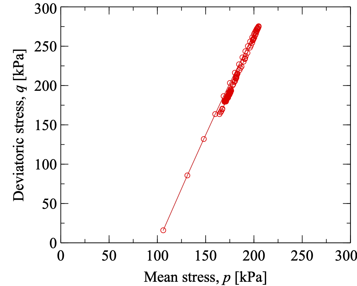
Then we can plot the stress-strain variation and the loading path as
shown in Figs. 3.9{reference-type=“ref”
reference=“figex2shearstress”} and
3.10{reference-type=“ref”
reference=“figex2shearpath”}.
Shearing.
Loading path during shearing.
During shearing, a series of states (i.e., files "shearxxx.xml.bz2")
has been saved sequentially so that it is readily to access other data
for post-processing, e.g., variation of mean coordination number,
anisotropy and so forth.
4 - Example 3: packing of GJKparticles
Here’s where your user finds out if your project is for them.
There are five kinds of shapes, namely sphere, polyhedron, cone,
cylinder and cuboid, in SudoDEM, for which the GJK algorithm of
contact detection is performed [^5], so that we coined a name
GJKparticle for grouping these particle shapes. In the Python module
_gjkparticle_utils (see Sec.
5.1.3{reference-type=“ref”
reference=“modgjkparticle”}), several construction functions are
provided including:
GJKSphere(radius,margin,mat)
GJKPolyhedron(vertices,extent,margin,mat, rotate)
GJKCone(radius, height, margin, mat, rotate)
GJKCylinder(radius, height, margin, mat, rotate)
GJKCuboid(extent, margin,mat, rotate)
Note: a margin is used to expand a particle for achieving a better
computational efficiency, which however should be large enough for
ensuring that collision occurs in this small region but small enough for
shape fidelity.
Similar to Example 1, we conduct some simulations of particles free
falling into a cubic box. We first import some modules:
#R: distance between two neighboring nodes#num_x: number of nodes along x axis#num_y: number of nodes along y axis#num_z: number of nodes along z axis#return a list of the postions of all nodesdefGridInitial(R,num_x=10,num_y=10,num_z=20):pos=list()foriinrange(num_x):forjinrange(num_y):forkinrange(num_z):x=i*R*2.0y=j*R*2.0z=k*R*2.0pos.append([x,y,z])returnpos
Set properties of materials:
1
2
3
4
5
6
7
8
p_mat=GJKParticleMat(label="mat1",Kn=1e4,Ks=7e3,frictionAngle=math.atan(0.5),density=2650,betan=0,betas=0)#define Material with default values#mat = GJKParticleMat(label="mat1",Kn=1e6,Ks=1e5,frictionAngle=0.5,density=2650) #define Material with default valueswall_mat=GJKParticleMat(label="wallmat",Kn=1e4,Ks=7e3,frictionAngle=0.0,betan=0,betas=0)#define Material with default valueswallmat_b=GJKParticleMat(label="wallmat",Kn=1e4,Ks=7e3,frictionAngle=math.atan(1),betan=0,betas=0)#define Material with default valuesO.materials.append(p_mat)O.materials.append(wall_mat)O.materials.append(wallmat_b)
Create the cubic box:
1
2
3
4
5
6
# create the box and add it to O.bodiesO.bodies.append(utils.wall(-R,axis=0,sense=1,material=wall_mat))#left wall along x axisO.bodies.append(utils.wall(2.0*R*num_x-R,axis=0,sense=-1,material=wall_mat))#right wall along x axisO.bodies.append(utils.wall(-R,axis=1,sense=1,material=wall_mat))#front wall along y axisO.bodies.append(utils.wall(2.0*R*num_y-R,axis=1,sense=-1,material=wall_mat))#back wall along y axisO.bodies.append(utils.wall(-R,axis=2,sense=1,material=wallmat_b))#bottom wall along z axis
Define engines and set a fixed time step:
1
2
3
4
5
6
7
8
9
10
11
12
13
newton=NewtonIntegrator(damping=0.3,gravity=(0.,0.,-9.8),label="newton",isSuperquadrics=4)O.engines=[ForceResetter(),InsertionSortCollider([Bo1_GJKParticle_Aabb(),Bo1_Wall_Aabb()],verletDist=0.2*0.01),InteractionLoop([Ig2_Wall_GJKParticle_GJKParticleGeom(),Ig2_GJKParticle_GJKParticle_GJKParticleGeom()],[Ip2_GJKParticleMat_GJKParticleMat_GJKParticlePhys()],# collision "physics"[GJKParticleLaw()]# contact law -- apply forces),newton]O.dt=1e-5
Polyhedral particles are generated as follows:
1
2
3
4
5
6
7
8
9
10
11
12
#generate a sampledefGenSample(r,pos):forpinpos:body=GJKPolyhedron([],[1.e-2,1.e-2,1.e-2],0.05*1e-2,p_mat,False)body.state.pos=pO.bodies.append(body)O.bodies[-1].shape.color=(rand.random(),rand.random(),rand.random())# create a lattice gridpos=GridInitial(R,num_x=num_x,num_y=num_y,num_z=num_z)# get positions of all nodes# create particles at each nodesGenSample(R,pos)#
{#figgjkpolyhedron width=“8cm”}
{#figgjkcone width=“8cm”}
For cones, we change the GenSample functions as follows:
1
2
3
4
5
6
7
#generate a sampledefGenSample(r,pos):forpinpos:body=GJKCone(0.005,0.01,0.05*1e-2,p_mat,False)body.state.pos=pO.bodies.append(body)O.bodies[-1].shape.color=(rand.random(),rand.random(),rand.random())
Fig. 3.12{reference-type=“ref” reference=“figgjkcone”}
shows final packing of cones without random initial orientations (i.e.,
the argument rotate is False). It can be seen that particles still
align in the lattice grid due to no disturbance in the tangential
direction.
Set the argument rotate to True as follows:
1
body=GJKCone(0.005,0.01,0.05*1e-2,p_mat,True)
{#figgjkcone2 width=“8cm”}
Rerun the simulation, and the initial particles have random
orientations. After free falling under gravity, it can be seen that the
lattice alignment corrupts, referring to Fig.
3.13{reference-type=“ref” reference=“figgjkcone2”}
{#figgjkcylinder width=“8cm”}
For cylindrical particles, the function GenSample is replaced as
follows:
Rerun the simulation, we obtain final packing of cylindrical particles
as shown in Fig. 3.14{reference-type=“ref”
reference=“figgjkcylinder”}, where it is evident that all particles stay
in a lattice grid after free falling. Again, we reset the argument
rotate to True so that all initial particles will have random
orientations.
1
body=GJKCylinder(0.005,0.01,0.05*1e-2,p_mat,True)
Rerun the simulation again, the column of cylindrical particles collapse
into the cubic box. The final state is visualized in Fig.
3.15{reference-type=“ref”
reference=“figgjkcylinder2”}.
{#figgjkcuboid width=“8cm”}
{#figgjkcuboid2 width=“8cm”}
We then continue two more simulations of cuboids. Change the function
GenSample as follows:
1
2
3
4
5
6
7
#generate a sampledefGenSample(r,pos):forpinpos:body=GJKCuboid([0.005,0.005,0.005],0.05*1e-2,p_mat,False)body.state.pos=pO.bodies.append(body)O.bodies[-1].shape.color=(rand.random(),rand.random(),rand.random())
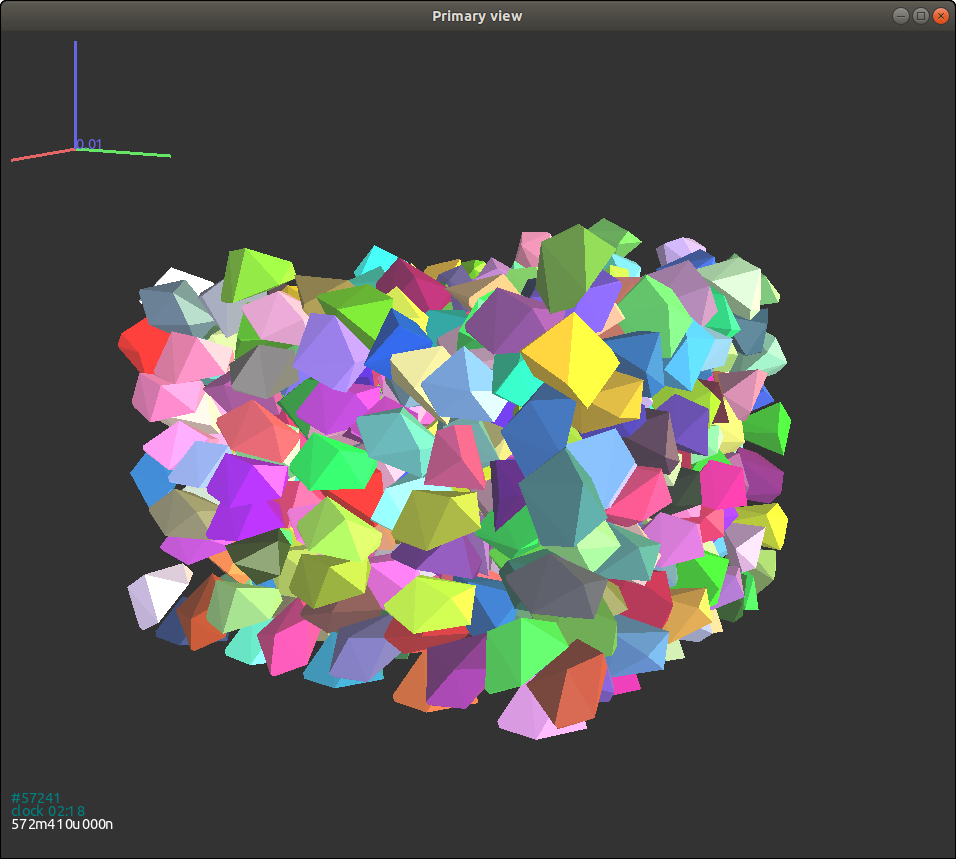
We obtain the final packing of cuboids without initial random
orientations as shown in Fig. 3.16{reference-type=“ref”
reference=“figgjkcuboid”}. Again, the alignment of particles remains a
lattice form. Rerun the simulation with the argument rotate setting to
True as follows:
The column of particles collapses but not too much due to small gaps
between particles.
5 - Example 4: packing of poly-superellipsoids
Here’s where your user finds out if your project is for them.
Poly-superellipsoid has a capability of capturing major features (e.g.,
flatness, asymmetry, and angularity) of realistic particles such as
sands in nature. A poly-superellipsoid is constructed by assembling
eight pieces of superellipoids, governed by the following surface
function at a local Cartesian coordinate system:
$$\Big(\big|\frac{x}{r_{x}}\big|^{\frac{2}{\epsilon_{1}}} + \big|\frac{y}{r_{y}}\big|^{\frac{2}{\epsilon_{1}}}\Big)^{\frac{\epsilon_{1}}{\epsilon_{2}}} +\big |\frac{z}{r_{z}}\big|^{\frac{2}{\epsilon_{2}}} = 1$$
with
where $r_x^+,r_y^+,r_z^+$ and $r_x^-,r_y^-,r_z^-$ are the principal
elongation along positive and negative directions of x, y, z axes,
respectively; $\epsilon_1, \epsilon_2$ control the squareness or
blockiness of particle surface, and their possible values are in $(0,2)$
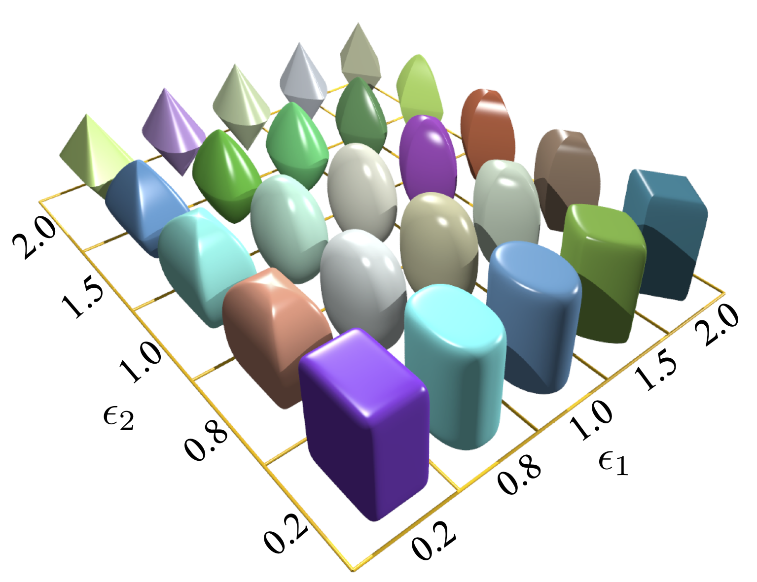
for convex shapes. Fig. 3.18{reference-type=“ref”
reference=“figmultipolysuper”} intuitively shows how $\epsilon_1$ and
$\epsilon_2$ affect particle surface. The module _superquadrics_utils
provides two functions to generate a poly-superellipsoid (see Sec.
5.1.2{reference-type=“ref”
reference=“modsuperquadrics”}):
#fromsudodem._superquadrics_utilsimport*importmathimportrandomimportnumpyasnpa=1.1734e-2isSphere=Falseap=0.4eps=0.5num_s=200num_t=8000trials=0wallboxsize=[10e-1,0,0]#size of the layer for the particles generationboxsize=np.array([7e-1,7e-1,20e-1])defdown():forbinO.bodies:if(isinstance(b.shape,PolySuperellipsoid)):if(len(b.intrs())==0):b.state.vel=[0,0,-2]b.state.angVel=[0,0,0]defgettop():zmax=0forbinO.bodies:if(isinstance(b.shape,PolySuperellipsoid)):if(b.state.pos[2]>=zmax):zmax=b.state.pos[2]returnzmaxdefGenparticles(a,eps,ap,mat,boxsize,num_s,num_t,bottom):globaltrialsgap=max(a,a*ap)#print(gap)num=0coor=[]width=(boxsize[0]-2.*gap)/2.length=(boxsize[1]-2.*gap)/2.height=(boxsize[2]-2.*gap)#iteration=0whilenum<num_sandtrials<num_t:isOK=Truepos=[0]*3pos[0]=random.uniform(-width,width)pos[1]=random.uniform(gap-length,length-gap)pos[2]=random.uniform(bottom+gap,bottom+gap+height)foriinrange(0,len(coor)):distance=sum([((coor[i][j]-pos[j])**2.)forjinrange(0,3)])if(distance<(4.*gap*gap)):isOK=Falsebreakif(isOK==True):coor.append(pos)num+=1trials+=1#print(num)returncoordefAddlayer(a,eps,ap,mat,boxsize,num_s,num_t):bottom=gettop()coor=Genparticles(a,eps,ap,mat,boxsize,num_s,num_t,bottom)forbincoor:#xyz = np.array([1.0,0.5,0.8,1.5,1.2,0.4])*0.1xyz=np.array([1.0,0.5,0.8,1.5,0.2,0.4])*0.1bb=NewPolySuperellipsoid([1.0,1.0],xyz,mat,True,isSphere)#bb.state.pos=[b[0],b[1],b[2]]bb.state.vel=[0,0,-1]O.bodies.append(bb)down()p_mat=PolySuperellipsoidMat(label="mat1",Kn=1e5,Ks=7e4,frictionAngle=math.atan(0.3),density=2650,betan=0,betas=0)#define Material with default valueswall_mat=PolySuperellipsoidMat(label="wallmat",Kn=1e6,Ks=7e5,frictionAngle=0.0,betan=0,betas=0)#define Material with default valueswallmat_b=PolySuperellipsoidMat(label="wallmat",Kn=1e6,Ks=7e5,frictionAngle=math.atan(1),betan=0,betas=0)#define Material with default valuesO.materials.append(p_mat)O.materials.append(wall_mat)O.materials.append(wallmat_b)O.bodies.append(utils.wall(-0.5*wallboxsize[0],axis=0,sense=1,material=wall_mat))#left xO.bodies.append(utils.wall(0.5*wallboxsize[0],axis=0,sense=-1,material=wall_mat))#right xO.bodies.append(utils.wall(-0.5*boxsize[1],axis=1,sense=1,material=wall_mat))#front yO.bodies.append(utils.wall(0.5*boxsize[1],axis=1,sense=-1,material=wall_mat))#back yO.bodies.append(utils.wall(0,axis=2,sense=1,material=wallmat_b))#bottom z#O.bodies.append(utils.wall(boxsize[0],axis=2,sense=-1, material = wallmat_b))#top znewton=NewtonIntegrator(damping=0.3,gravity=(0.,0.,-9.8),label="newton",isSuperquadrics=2)#isSuperquadrics=2 for Poly-superellipsoidsO.engines=[ForceResetter(),InsertionSortCollider([Bo1_PolySuperellipsoid_Aabb(),Bo1_Wall_Aabb()],verletDist=0.2*0.1),InteractionLoop([Ig2_Wall_PolySuperellipsoid_PolySuperellipsoidGeom(),Ig2_PolySuperellipsoid_PolySuperellipsoid_PolySuperellipsoidGeom()],[Ip2_PolySuperellipsoidMat_PolySuperellipsoidMat_PolySuperellipsoidPhys()],# collision "physics"[PolySuperellipsoidLaw()]# contact law -- apply forces),newton]O.dt=5e-5#adding particlesAddlayer(a,eps,ap,p_mat,boxsize,num_s,num_t)#Note: these particles may intersect with each other when we generate them.#setting the Display properties. You can go to the Display panel to set them directly.sudodem.qt.Gl1_PolySuperellipsoid.wire=Falsesudodem.qt.Gl1_PolySuperellipsoid.slices=10sudodem.qt.Gl1_Wall.div=0#hide the walls
After running the script above, the user is expected to see a packing as
shown in Fig. 3.19{reference-type=“ref”
reference=“figpolysuperpacking”}.
{#figpolysuperpacking
width=“10cm”}
6 - Example 5: packing of superellipses
Here’s where your user finds out if your project is for them.
The surface function of a superellipse in the local Cartesian
coordinates can be defined as
$$\big|\frac{x}{r_x}\big|^{\frac{2}{\epsilon}} + \big|\frac{y}{r_y}\big|^{\frac{2}{\epsilon}} = 1$$
where $r_x$ and $r_y$ are referred to as the semi-major axis lengths in
the direction of x, and y axies, respectively; and $\epsilon \in (0, 2)$
is the shape parameters determining the sharpness of particle edges or
squareness of particle surface. Here we simulate packing of
superellipses under gravity with the following script:
 {#figgjkpolyhedron width=“8cm”}
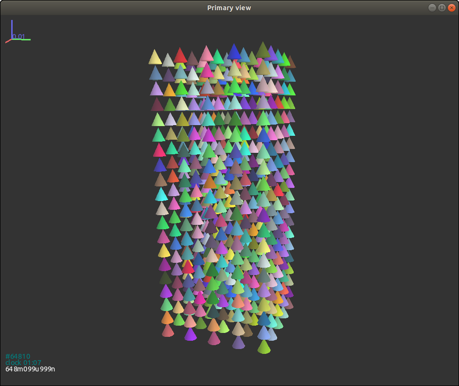 {#figgjkcone width=“8cm”}
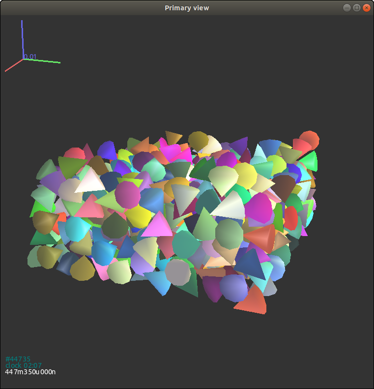 {#figgjkcone2 width=“8cm”}
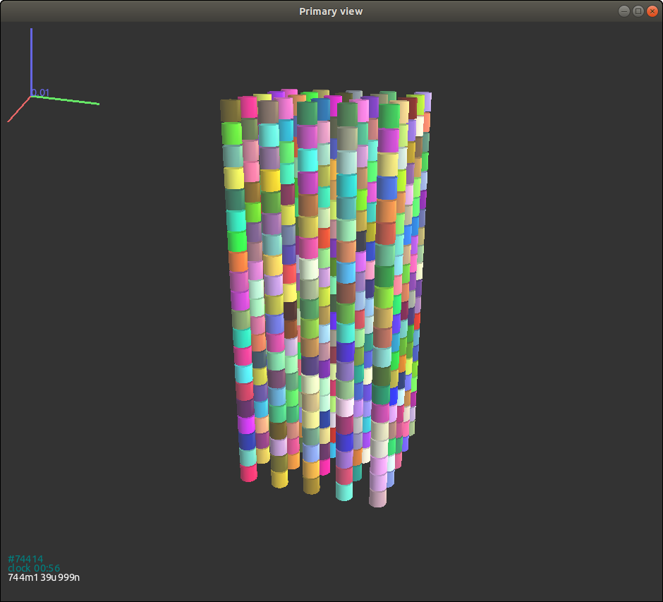 {#figgjkcylinder width=“8cm”}
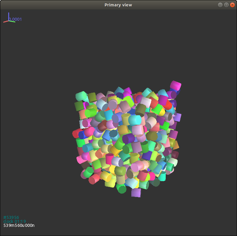 {#figgjkcylinder2 width=“8cm”}
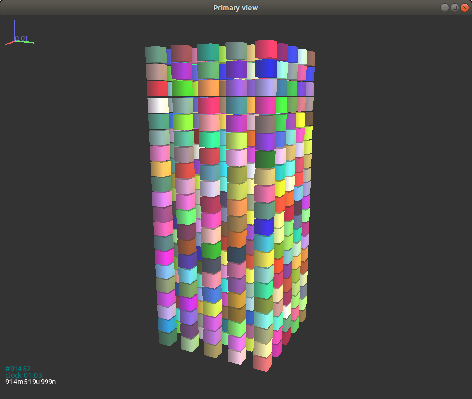 {#figgjkcuboid width=“8cm”}
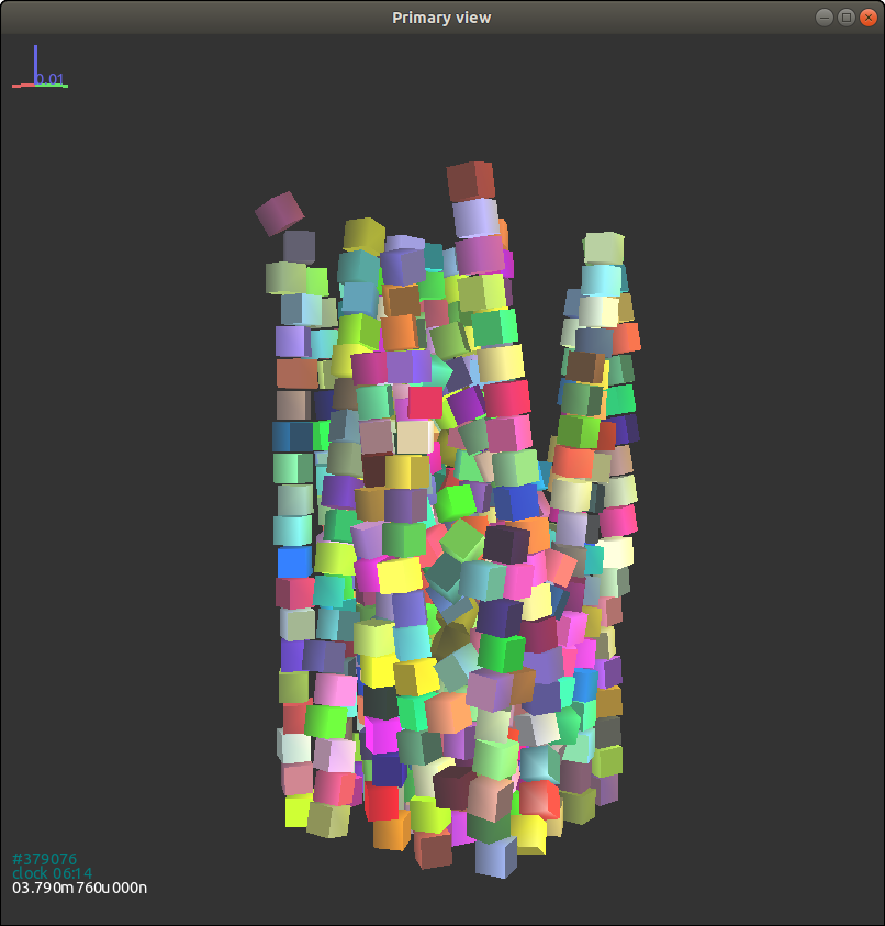 {#figgjkcuboid2 width=“8cm”}
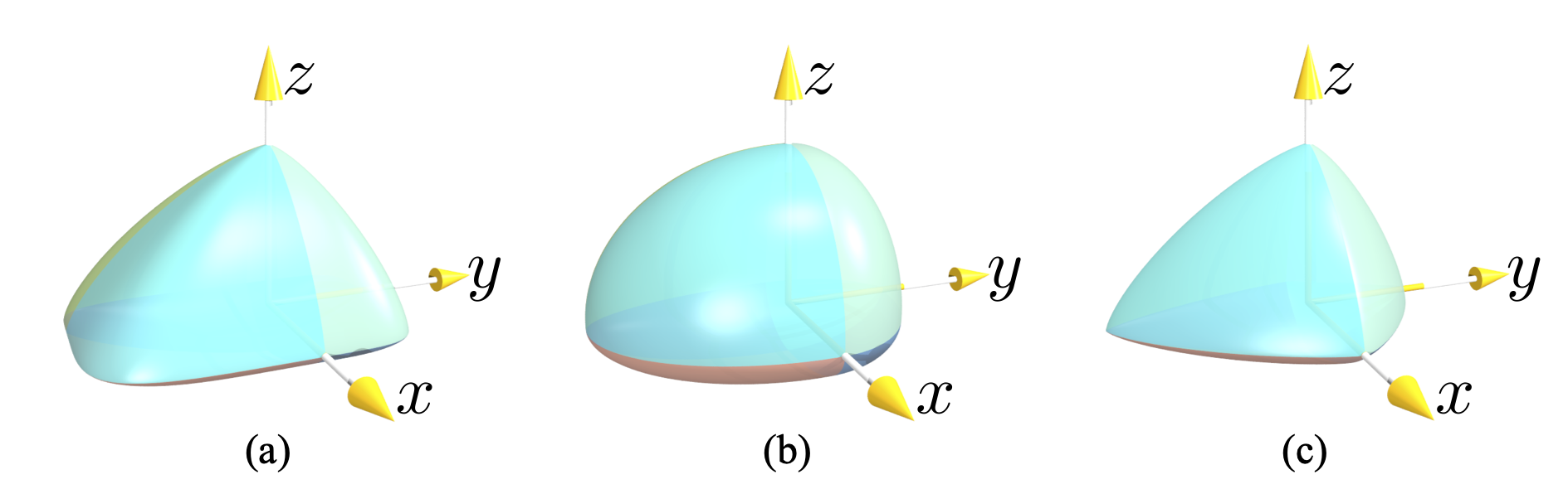 Poly-superellipsoids with
$r_x^+=1.0, r_x^-=0.5, r_y^+=0.8, r_y^- = 0.9, r_z^+ = 0.4, r_z^- = 0.6$
and (a) $\epsilon_1=0.4, \epsilon_2=1.5$, (b)
$\epsilon_1=\epsilon_2=1.0$, (c)
$\epsilon_1=\epsilon_2=1.5$.
Poly-superellipsoids with
$r_x^+=1.0, r_x^-=0.5, r_y^+=0.8, r_y^- = 0.9, r_z^+ = 0.4, r_z^- = 0.6$
and (a) $\epsilon_1=0.4, \epsilon_2=1.5$, (b)
$\epsilon_1=\epsilon_2=1.0$, (c)
$\epsilon_1=\epsilon_2=1.5$.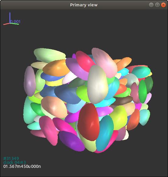 {#figpolysuperpacking
width=“10cm”}
{#figpolysuperpacking
width=“10cm”}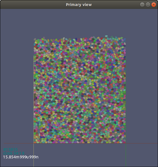 {#figpackingellipse width=“10cm”}