 1
 2
 3
 4
 5
 6
 7
 8
 9
10
11
12
13
14
15
16
17
18
19
20
21
22
23
24
25
26
27
28
29
30
31
32
33
34
35
36
37
38
39
40
41
42
43
44
45
46
47
48
49
50
51
52
53
54
55
56
57
58
59
60
61
62
63
64
65
66
67
68
69
70
71
72
|
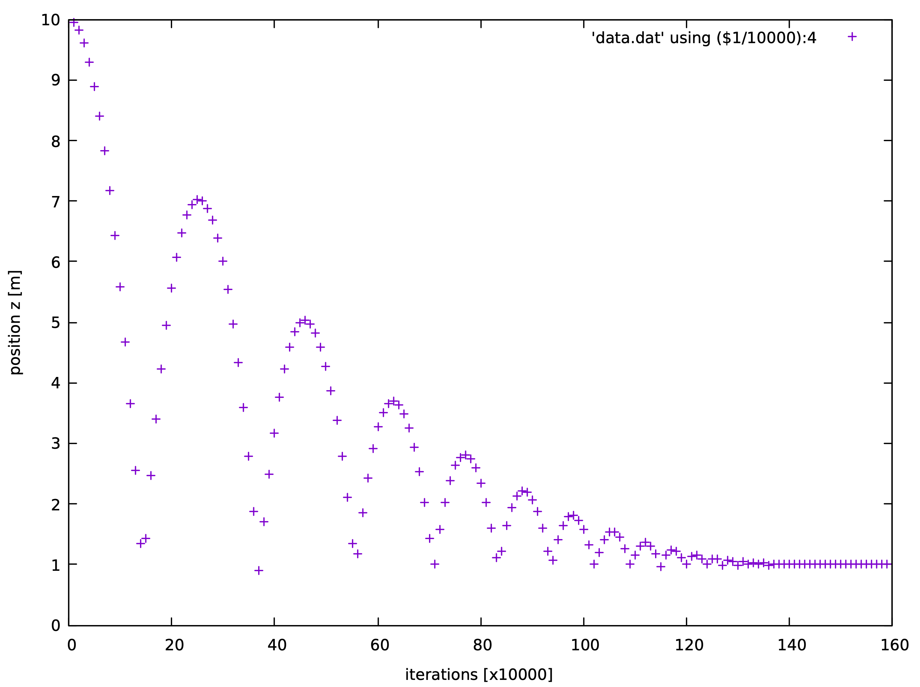
# A sphere free falling on a ground under gravity

from sudodem import utils # module utils has some auxiliary functions

#1. we define materials for particles
mat = RolFrictMat(label="mat1",Kn=1e8,Ks=7e7,frictionAngle=math.atan(0.0),density=2650) # material 1 for particles
wallmat1 = RolFrictMat(label="wallmat1",Kn=1e8,Ks=0,frictionAngle=0.) # material 2 for walls

# we add the materials to the container for materials in the simulation.
# O can be regarded as an object for the whole simulation.
# We can see that materials is a property of O, so we use a dot operation (O.materials) to get the property (materials).
O.materials.append(mat) # materials is a list, i.e., a container for all materials involving in the simulations
O.materials.append(wallmat1)
# adding a material to the container (materials) so that we can easily access it by its label. See the definition of a wall below.

#create a spherical particle
sp = sphere((0,0,10.0),1.0, material = mat)
O.bodies.append(sp)
# create the ground as an infinite plane wall
ground = utils.wall(0,axis=2,sense=1, material = 'wallmat1') # utils.wall defines a wall with normal parallel to one axis of the global Cartesian coordinate system. The first argument (here = 0) specifies the location of the wall, and with the keyword axis (here = 2, axis has a value of 0, 1, 2 for x, y, z axies respectively) we know that the normal of the wall is along z axis with centering at z = 0 (0, specified by the first argument); the second keyword sense (here = 1, sense can be -1, 0, 1 for negative, both, and positive sides respectively) specifies that the positive side (i.e., the normal points to the positive direction of the axis) of the wall is activated, at which we will compute the interaction of a particle and this wall; the last keyword materials specifies a material to this wall, and we assign a string (i.e., the label of wallmat1) to the keyword, and directly assigning the object of the material (i.e., wallmat1 returned by RolFrictMat) is also acceptable.
O.bodies.append(ground) # add the ground to the body container


# define a function invoked periodically by a PyRunner
def record_data():
    #open a file
    fout = open('data.dat','a') #create/open a file named 'data.dat' in append mode
    #we want to record the position of the sphere
    p = O.bodies[0] # the sphere has been appended into the list O.bodies, and we can use the corresponding index to access it. We have added two bodies in total to O.bodies, and the sphere is the first one, i.e., the index is 0.
    # p is the object of the sphere
    # as a body object, p has several properties, e.g., state, material, which can be listed by p.dict() in the commandline.
    pos = p.state.pos # get the position of the sphere
    print>>fout, O.iter, pos[0], pos[1], pos[2] # we print the iteration number and the position (x,y,z) into the file fout.
    # then, close the file and release resource
    fout.close()

# create a Newton engine by which the particles move under Newton's Law
newton=NewtonIntegrator(damping = 0.1,gravity=(0.,0.0,-9.8),label="newton")
# we set a local damping of 0.1 and gravitational acceleration -9.8 m/s2 along z axis.

# the engine container is the kernel part of a simulation
# During each time step, each engine will run one by one for completing a DEM cycle.
O.engines=[
   ForceResetter(), # first, we need to reset the force container to store upcoming contact forces
   # next, we conduct the broad phase of contact detection by comparing axis-aligned bounding boxs (AABBs) to rule out those pairs that are definitely not contacting.
   InsertionSortCollider([Bo1_Sphere_Aabb(),Bo1_Wall_Aabb()],verletDist=0.2*0.01),
   # then, we execute the narrow phase of contact detection
   InteractionLoop( # we will loop all potentially contacting pairs of particles
	  [Ig2_Sphere_Sphere_ScGeom(), Ig2_Wall_Sphere_ScGeom()], # for different particle shapes, we will call the corresponding functions to compute the contact geometry, for example, Ig2_Sphere_Sphere_ScGeom() is used to compute the contact geometry of a sphere-sphere pair.
	  [Ip2_RolFrictMat_RolFrictMat_RolFrictPhys()], # we will compute the physical properties of contact, e.g., contact stiffness and coefficient of friction, according to the physical properties of contacting particles.
	  [RollingResistanceLaw(use_rolling_resistance=False)]   # Next, we compute contact forces in terms of the contact law with the info (contact geometric and physical properties) computed at last two steps.
   ),
   newton, # finally, we compute acceleration and velocity of each particle and update their positions.
   #at each time step, we have a PyRunner function help to hack into a DEM cycle and do whatever you want, e.g., changing particles' states, and saving some data, or just stopping the program after a certain running time.
   PyRunner(command='record_data()',iterPeriod=10000,label='record',dead = False)
]

# we need to set a time step
O.dt = 1e-5

# clean the file data.dat and write a file head
fout = open('data.dat','w') # we open the file in a write mode so that the file will be clean
print>>fout, 'iter, x, y, z' # write a file head
fout.close() # close the file

# run the simulation
# you have two choices:
# 1. give a command here, like,
# O.run()
# you can set how many iterations to run
O.run(1600000)
# 2. clike the run button at the GUI controler
|