Example 2: triaxial tests of super-ellipsoids
This example shows a triaxial compression simulation of superellipsoids using an Engine CompressionEngine. The users can also customized their engines or compression procedures easily via a PyRunner Engine. Here is a basic setup of CompressionEngine for consolidation and compression below.
-
Consolidation
1 2 3 4 5 6 7 8 9 10 11 12 13 14 15triax=CompressionEngine( goalx = 1.0e5, # confining stress 100 kPa goaly = 1.0e5, goalz = 1.0e5, savedata_interval = 10000, echo_interval = 2000, continueFlag = False, max_vel = 100.0, gain_alpha = 0.5, f_threshold = 0.01, #1-f/goal fmin_threshold = 0.01, #the ratio of deviatoric stress to mean stress unbf_tol = 0.01, #unblanced force ratio file='record-con' )-
goalx = goaly = goalz = confining stress
-
savedata_interval: the interval of DEM iterations for saving some data (Axial Strain, Volumetric Strain, Mean Stress and DeviatorStress) into a file specified by file. Deprecated for consolidation.
-
echo_interval: the interval of DEM iterations for outputting information (Iterations, Unbalanced force ratio, stresses in x, y, z directions) in the terminal
-
continueFlag: reserved keyword for continuing consolidation or compression.
-
max_vel: the maximum velocity of a wall, which is useful to constrain the movement of a wall during confining.
-
gain_alpha $\alpha$: guiding the movement of the confining walls. $$v_w = \alpha \frac{f_w - f_g}{\Delta t \sum k_n}$$ where $v_w$ is the velocity of a confining wall at the next time step; $f_w$ and $f_g$ are the present and goal confining forces, respectively; $\Delta t$ is the time step, and $\sum k_n$ is the summation of normal contact stiffness from all particle-wall contacts on this wall.
-
f_threshold $\alpha_f$: a target ratio of the deviation of the present stress from the goal to the goal, i.e., $$\alpha_f = \frac{|f_w-f_g|}{f_g}$$
-
fmin_threshold $\beta_f$: a target ratio of the deviatoric stress $q$ to the mean stress $p$, i.e., $$\beta_f = \frac{q}{p},\quad p= \frac{\sigma_{ii}}{3},\quad q=\sqrt{\frac{3}{2}\sigma_{ij}^{'}\sigma_{ij}^{'}}$$ $$\sigma_{ij} = \frac{1}{V}\sum_{c\in V}f_i^cl_j^c,\quad \sigma_{ij}^{'}=\sigma_{ij}-p\delta_{ij}$$ where $\sigma_{ij}$ is the stress tensor with an assembly, and $\sigma_{ij}^{'}$ is its corresponding deviatoric part; $V$ is the total volume of the specimen; $f^c$ and $l^c$ are the contact force and branch vector at contact $c$, respectively, and $\delta_{ij}$ is the Kronecker delta.
-
unbf_tol $\gamma_f$: a target unbalanced force ratio defined as $$\gamma_f = \frac{\sum\limits_{B_i\in V} |\sum\limits_{j\in B_i}f^c_j+f^b_j|}{2\sum\limits_{c\in V}|f^c|}$$ Note: the consolidation ends up with that all $\alpha_f$, $\beta_f$ and $\gamma_f$ reach the targets.
-
file: the file name for the recording file
-
-
Compression
1 2 3 4 5 6 7 8 9 10 11 12 13 14 15 16triax=CompressionEngine( z_servo = False, goalx = 1.0e5, goaly = 1.0e5, goalz = 0.01, ramp_interval = 10, ramp_chunks = 2, savedata_interval = 1000, echo_interval = 2000, max_vel = 10.0, gain_alpha = 0.5, file='sheardata', target_strain = 0.4, gain_alpha = 0.5 )-
z_servo: a False value will trigger a strain (or displacement) control in the z direction, and in this case goalz needs a strain rate.
-
ramp_interval: iterations needed for reaching a constant strain rate. This keyword is designed to mimic a continuing loading at laboratory, but it seems not too valued and setting a small value to kindly deprecate it.
-
ramp_chunks: number of intervals to reach the constant strain rate combined with the keyword ramp_interval. It will be deprecated as does ramp_interval.
-
target_strain: at this level of strain the shear procedures ends. The strain is ogarithmic strain.
Note: to ensure quasi-static behavior during shear, the shear strain rate should be sufficiently small. Specifically, the inertial number $I$ should be maintained less than $10^{-3}$ $$I = \dot{\epsilon_1}\frac{\hat{d}}{\sqrt{\sigma_0/\rho}}$$ where $\dot{\epsilon_1}=\mathrm{d}\epsilon_1/\mathrm{d}t$ is the major principal strain rate; $\hat{d}$ and $\rho$ are the average diameter and material density of particles respectively; $\sigma_0$ is the confining stress.
-
As a demonstration, we first give an example of consolidation as follows:
|
|
The output in the terminal is akin to the follows:
calm procedure is over
0 particles are deleted!
consolidation begins
Iter 50000 Ubf 0.483161, Ss_x:9.67986e-05, Ss_y:4.15364e-05, Ss_z:6.1184e-05, e:0.992618
Iter 52000 Ubf 0.461741, Ss_x:1.2412, Ss_y:1.06812, Ss_z:1.10116, e:0.854445
Iter 54000 Ubf 0.263699, Ss_x:1.75334, Ss_y:1.98567, Ss_z:1.62181, e:0.757469
Iter 56000 Ubf 0.118329, Ss_x:3.06302, Ss_y:3.54818, Ss_z:3.22986, e:0.679106
Iter 58000 Ubf 0.0110747, Ss_x:22.0177, Ss_y:21.3303, Ss_z:21.3485, e:0.614824
Iter 60000 Ubf 0.000577066, Ss_x:91.4199, Ss_y:89.6039, Ss_z:89.1057, e:0.58984
Iter 62000 Ubf 0.000128293, Ss_x:100.012, Ss_y:99.7251, Ss_z:99.6123, e:0.587807
consolidation completed!
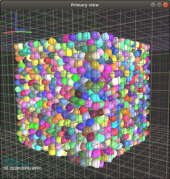
After consolidation (see the snapshot in Fig. 3.7{reference-type=“ref” reference=“figex2consol”}), we obtain a state file by
|
|
Then, the consolidated assembly is subjected to triaxial compression with the following scripts.
|
|
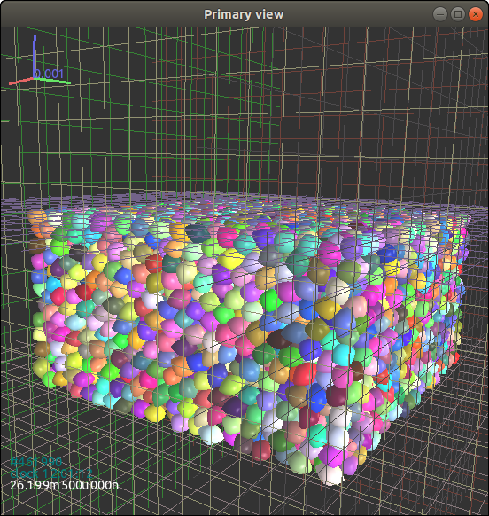
The compression ends up with an axial strain of 40%, and the final configuration of particles is shown in Fig. 3.8{reference-type=“ref” reference=“figex2shear”}.
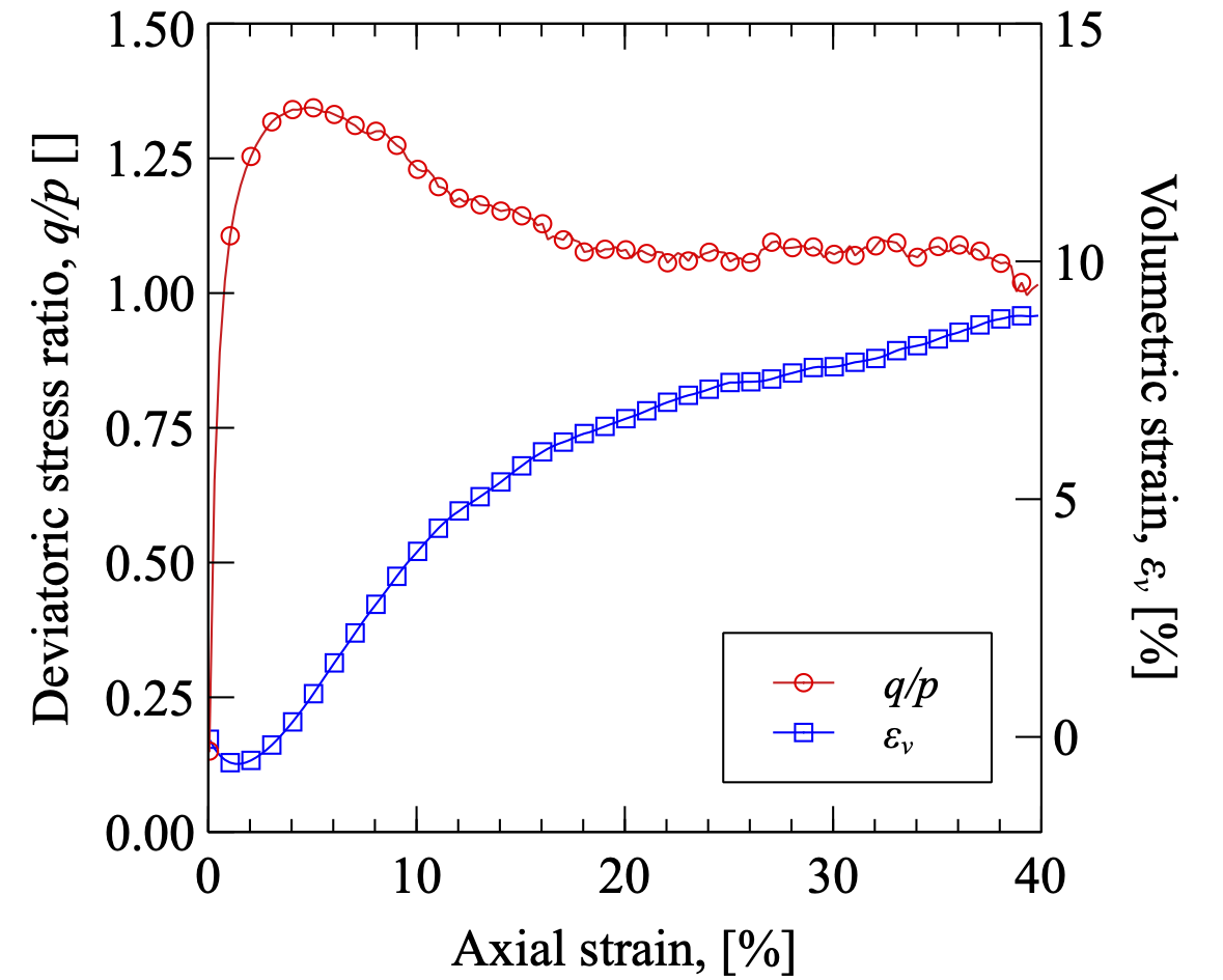
The macroscopic mechanical response of a granular material during shearing can be quantified by the stress tensor that is calculated from discrete measurements with the following definition: $$\label{eqDEMstress} \sigma_{ij} = \frac{1}{V} \sum_{c \in V} f_i^c l_j^c$$ where $V$ is the total volume of the assembly, $f^c$ is the contact force at the contact $c$, and $l^c$ is the branch vector joining the the centres of the two contacting particles at contact $c$. The mean stress $p$ and the deviatoric stress $q$ are defined as: $$p = \frac{1}{3}\sigma_{ii},\quad q = \sqrt{\frac{3}{2} \sigma_{ij}^{'}\sigma_{ij}^{'}}$$ where $\sigma_{ij}^{'}$ is the deviatoric part of stress tensor $\sigma_{ij}$.
Given that the cubical specimens are confined by rigid walls, the axial strain $\epsilon_z$ and the volumetric strain $\epsilon_v$ can be approximately calculated from the positions of the boundary walls, i.e., $$\epsilon_z = \int_{H_0}^{H}\frac{\mathrm{d}h}{h}=-\ln\frac{H_0}{H},\quad \epsilon_v = \epsilon_x+\epsilon_y+\epsilon_z=\int_{V_0}^{V}\frac{\mathrm{d}v}{v}=-\ln\frac{V_0}{V}$$ where $H$ and $V$ are the height and volume of the specimen during shearing, respectively, and $H_0$ and $V_0$ are their initial values before shear. Positive values of volumetric strain represent dilatancy.
The recorded data ‘sheardata’ looks like below:
AxialStrain VolStrain meanStress deviatorStress
0.000511000266 0.000490480823 106090.98 15931.56
0.003011001516 0.002450117535 131061.41 85718.91
0.005511002766 0.003867756447 148076.65 131980.95
0.008011004016 0.004825115794 159924.28 163706.90
0.010511005266 0.005409561745 168606.27 186520.14
0.013011006516 0.005673777079 175131.53 203243.28
0.015511007766 0.005650846281 180293.19 216248.17
0.018011009016 0.005393122254 184581.23 227010.23
Then we can plot the stress-strain variation and the loading path as shown in Figs. 3.9{reference-type=“ref” reference=“figex2shearstress”} and 3.10{reference-type=“ref” reference=“figex2shearpath”}.
Shearing.
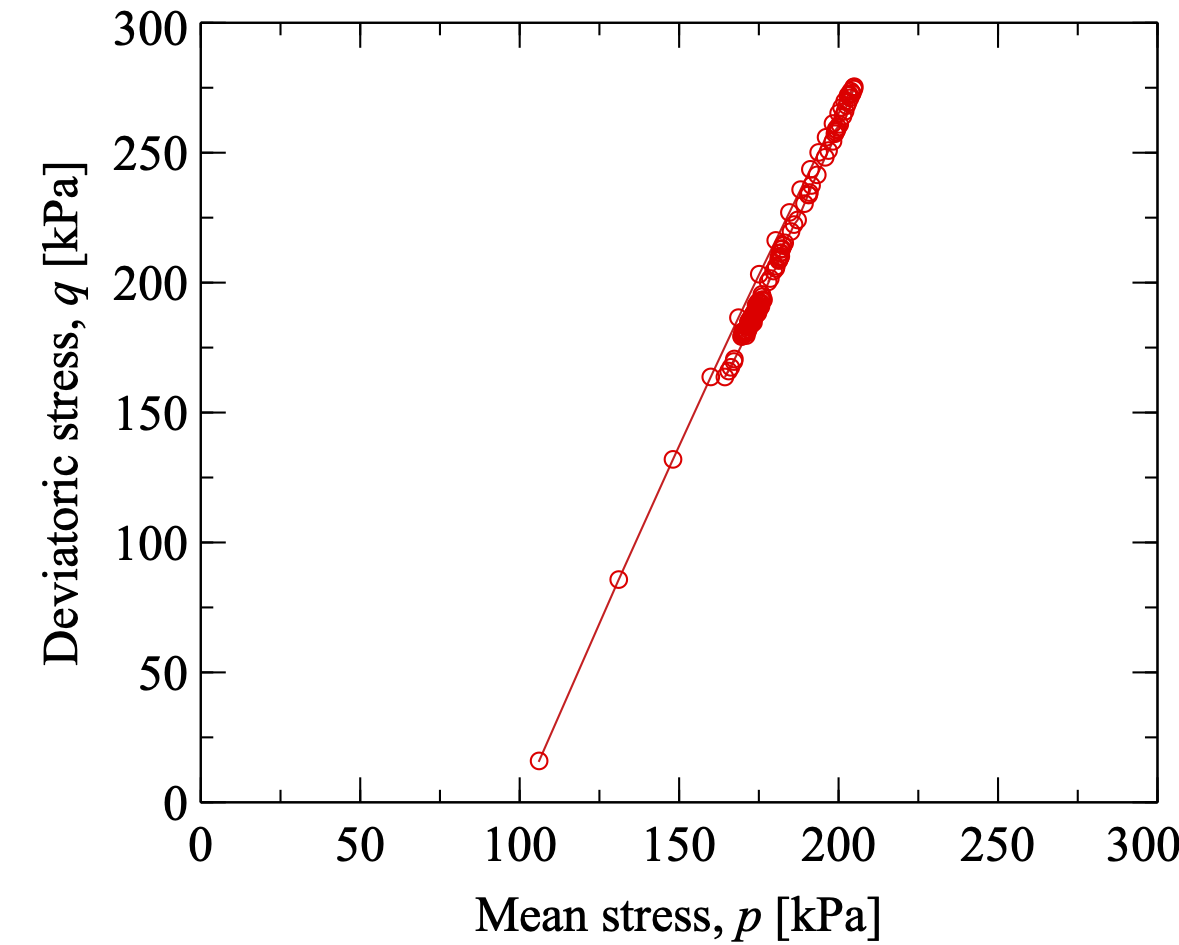
Loading path during shearing.
During shearing, a series of states (i.e., files "shearxxx.xml.bz2") has been saved sequentially so that it is readily to access other data for post-processing, e.g., variation of mean coordination number, anisotropy and so forth.