SudoDEM
- 1: 必备条件
- 2: 示例
- 2.1: 示例 0: 运行一个简单的模拟
- 2.2: 示例 1: 超级椭球堆积模拟
- 2.3: 示例 2: 超级椭球三轴试验模拟
- 2.4: 示例 3: GJK颗粒的堆积模拟
- 2.5: 示例 4: 组合超级椭球的堆积模拟
- 2.6: 示例 5: 超椭圆堆积模拟
- 3: 后处理
- 4: Python类参考文档
1 - 必备条件
我们假定用户已经预装Linux操作系统(推荐安装Ubuntu 14-18)以及Python(2.7)和一些基本Python库(例如numpy), 其他第三方库(例如Boost和Qt)可以在稍后进行安装。
基本的Linux操作命令
用户仅需掌握少许Linux基本命令即可开始SudoDEM的安装和使用。
Linux基本命令(参见下文)可使用命令行执行,命令行的开启可使用快捷键 “CTRL+ALT+T” 或者使用系统菜单。
-
sudo apt-get install package[^2]: 该命令可用于使用超级用户权限为系统安装对应名字的库。
-
pwd: 该命令可用于打印当前命令行的工作路径。
-
cd directory:该命令用于切换命令行的工作文件夹路径,文件夹路径可以是相对或者绝对路径。此处我们别介绍两个特别的文件夹路径名字,即 ‘.’ 和 ‘..'。’.' 表示当前文件夹路径,'..‘表示当前文件夹的上一层文件夹路径,这两种路径名字都属于相对文件夹路径,方便用户轻松切换路径。例如 ' cd ../sub’ 将会切换到与当前文件夹路径同级的另一个叫做 ‘sub’ 的文件夹。而 ‘cd /home/user’ 则会切换到当前登录用户家目录文件夹下。
-
prog 或 ./path/prog: 该命令用于执行一个名为 prog 的程序。如果该程序处于命令行搜索路径下,则键入 prog 即可成功执行;若该程序不在命令行搜索路径下,则需要在指定该程序所处的相对或绝对路径后才可成功执行。
-
‘CTRL+C’: 该命令用于终止一个正在命令行运行的程序。
    $> sudo apt-get install python-numpy
    $> pwd
    $> cd /home/
    $> sudodem3d
Python 2.7
Python是缩进敏感型程序,缩进帮助Python进行作用域的划分。'#' 符号用于Python代码的单行注释。下面的代码给出了Python的一些基本的语法结构:
|
|
恭喜你!你现在已经掌握了运行数值模拟所必要的全部知识!
但也许这对于好学的你来说还不够!你可能会好奇更多酷炫的技术,比如如何进行文件的读写操作,如何利用Python进行面向对象编程。别急,我们后续教程会逐步为你呈现!
库的安装
SudoDEM 托管于GitHub 请点击这里。 我们将会给出两种 SudoDEM 的安装方式方便大家选择。
二进制安装
第一步: 获取安装包[^3]
你可以从这里下载已经编译好的 SudoDEM 二进制程序 , 然后将该二进制包解压到任意文件夹 (例如, /home/xxx/)。 如果你已经下载了 SudoDEM 主程序,但是没有包含对应的第三方库,你需要再下载 "3rdlibs.tar.xz" 并将其解压在 SudoDEM 子文件夹 "lib" 中。你可以参考下文所示的 SudoDEM 文件结构:
::: {.forest} for tree= font=, grow'=0, child anchor=west, parent anchor=south, anchor=west, calign=first, inner xsep=7pt, edge path= (!u.south west) +(7.5pt,0) |- (.child anchor) pic folder ; , file/.style=edge path=(!u.south west) +(7.5pt,0) |- (.child anchor) ;, inner xsep=2pt,font= , before typesetting nodes= if n=1 insert before=[,phantom] , fit=band, before computing xy=l=15pt, [/home/xxx/SudoDEM/ [bin/ [sudodem3d] ] [lib/ [3rdlibs/] [sudodem/] ] [share/ ] ] :::
第二步: 设置环境变量 PATH
将 sudodem3d 安装路径(例如,'/home/xxx/SudoDEM/bin')添加到环境变量配置文件中(例如,'/home/xxx/.bashrc'):
PATH=${PATH}:/home/xxx/SudoDEM/bin
不使用超级用户权限的 sudodem3d 源代码编译安装
下面的视频也许会帮助你完成 sudodem3d 的源代码编译安装(注:用户可以直接复制视频中的命令)。
(1) 文件夹结构
在源代码文件解压后,你将会看到如下文件夹结构
./home/xxx/SudoDEM
- [SudoDEM2D]
- [SudoDEM3D]
- [scripts]
- [INSTALL]
- [LICENSE]
- [Readme.md]
::: {.forest} for tree= font=, grow'=0, child anchor=west, parent anchor=south, anchor=west, calign=first, inner xsep=7pt, edge path= (!u.south west) +(7.5pt,0) |- (.child anchor) pic folder ; , file/.style=edge path=(!u.south west) +(7.5pt,0) |- (.child anchor) ;, inner xsep=2pt,font= , before typesetting nodes= if n=1 insert before=[,phantom] , fit=band, before computing xy=l=15pt, [/home/xxx/SudoDEM [SudoDEM2D ] [SudoDEM3D ] [scripts] [INSTALL,file ] [LICENSE,file ] [Readme.md,file ] ] :::
用户可以添加子文件夹, 例如, ‘3rdlib’, ‘build2d’, ‘build3d’和 ‘sudodeminstall’到 ‘SudoDEM’ 文件夹中。现在文件夹结构将会被更新如下:
::: {.forest} for tree= font=, grow’=0, child anchor=west, parent anchor=south, anchor=west, calign=first, inner xsep=7pt, edge path= (!u.south west) +(7.5pt,0) |- (.child anchor) pic folder ; , file/.style=edge path=(!u.south west) +(7.5pt,0) |- (.child anchor) ;, inner xsep=2pt,font= , before typesetting nodes= if n=1 insert before=[,phantom] , fit=band, before computing xy=l=15pt, [/home/xxx/SudoDEM [SudoDEM2D ] [SudoDEM3D ] [3rdlib] [build2d] [build3d] [sudodeminstall] [scripts] [INSTALL,file ] [LICENSE,file ] [Readme.md,file ] ] :::
子文件夹 ‘3rdlib’ 用于存放第三方库的文件。需要注明的是该文件夹不仅存放第三方库的头文件,同时还将存放第三方库库编译后的动态链接库文件 ('*.so.*')。 在 ‘SudoDEM’ 编译完成后,用户需要手动将 ‘SudoDEM’ 所依赖的所有第三方库的对应文件拷贝到子文件夹 ‘3rdlib’ 中。‘SudoDEM’ 的二维和三维版本的编译分别在 ‘build2d’ 和 ‘build3d’ 中进行,编译后的所有生成文件将会被安装在 ‘sudodeminstall’ 文件夹中。
(2) 编译第三方库
::: {.forest} for tree= font=, grow’=0, child anchor=west, parent anchor=south, anchor=west, calign=first, inner xsep=7pt, edge path= (!u.south west) +(7.5pt,0) |- (.child anchor) pic folder ; , file/.style=edge path=(!u.south west) +(7.5pt,0) |- (.child anchor) ;, inner xsep=2pt,font= , before typesetting nodes= if n=1 insert before=[,phantom] , fit=band, before computing xy=l=15pt, [/home/xxx/SudoDEM/3rdlib [boost-1_6_7] [eigen3.3.5] [libQGLViewer-2.6.3] [minieigen] ] :::
主要第三方依赖库:
-
Boost-1.67
从 Boost 官方网站下载对应的源代码文件 (https://www.boost.org/users/history/version_1_67_0.html) 或者可以选择从 github 下载 (https://github.com/SwaySZ/boost-1_6_7)。cd boost-1\_6\_7 ./bootstrap.sh --prefix=$PWD/../boost167 --with-libraries=python,thread,filesystem,iostreams,regex,serialization,system,date_time link=shared runtime-link=shared --without-icu ./b2 -j3 ./b2 install -
Eigen-3.3.5: 无需安装但需要包含所有的头文件。 用户可以选择从我们提供的 github 仓库来下载 (https://github.com/SwaySZ/Eigen-3.3.5).
-
MiniEigen
github 仓库下载地址 (https://github.com/SwaySZ/minieigen). 在 CMakeLists.txt' 设置已经编译好的 Boost 的路径:set(BOOST_ROOT "/home/swayzhao/software/DEM/3rdlib/boost167")然后执行,
mkdir build
cd build
cmake ../
make
编译完成后请拷贝文件 ‘minieigen.so’ 到 SudoDEM 子文件夹 ‘lib/3rdlibs/py’ 下面。
-
LibQGLViewer-2.6.3
从 github 仓库下载对应的源代码 (https://github.com/SwaySZ/libQGLViewer-2.6.3)cd QGLViewer qmake make
其他工具和依赖库:
-
biuld-essential, cmake
-
freeglut3-dev
-
zlib1g-dev (boost)
-
python-dev (boost)
-
pyqt4-dev-tools
-
qt4-default
-
python-numpy python-tk
-
libbz2-dev
-
python-xlib python-qt4
-
ipython3.0 python-matplotlib
-
libxi-dev
-
libglib2.0-dev
-
libxmu-dev
(3) 编译 SudoDEM 主程序
我们将在这一小节给出 SudoDEM3D 的编译示例。编译前请确认你的文件夹结构如下:
::: {.forest} for tree= font=, grow'=0, child anchor=west, parent anchor=south, anchor=west, calign=first, inner xsep=7pt, edge path= (!u.south west) +(7.5pt,0) |- (.child anchor) pic folder ; , file/.style=edge path=(!u.south west) +(7.5pt,0) |- (.child anchor) ;, inner xsep=2pt,font= , before typesetting nodes= if n=1 insert before=[,phantom] , fit=band, before computing xy=l=15pt, [/home/xxx/SudoDEM/SudoDEM3D [cMake] [CMakeLists.txt, file] [core] [doc] [gui] [lib] [pkg] [py] ] :::
编译前用户需要修改 ‘CMakeLists.txt’ 用于 SudoDEM 安装路径以及第三方依赖库的路径设置。
(a) 设置安装路径:
SET(CMAKE_INSTALL_PREFIX "${CMAKE_CURRENT_SOURCE_DIR}/../sudodeminstall/SudoDEM3D")
(b) 设置 Boost 库的路径:
set(BOOST_ROOT "${CMAKE_CURRENT_SOURCE_DIR}/../3rdlib/boost167")
(c) QGLViewer 的头文件以及动态链接库通过下面两行来设置:
set(QGLVIEWER_INCLUDE_DIR "${CMAKE_CURRENT_SOURCE_DIR}/../3rdlib/libQGLViewer-2.6.3/")
set(QGLVIEWER_LIBRARIES "${CMAKE_CURRENT_SOURCE_DIR}/../3rdlib/libQGLViewer-2.6.3/QGLViewer/libQGLViewer.so")
(d) 拷贝已经安装完成的 numpy 和 pyqt4 文件到 SudoDEM 子文件夹 ‘./lib/3rdlibs/py’。你也许需要修改 cmake 的配置文件 FindNumPy.cmake 用于 numpy 的路径搜索:
set(DPDIR "${CMAKE_CURRENT_SOURCE_DIR}/../dem2dinstall/SudoDEM/lib/3rdlibs/py/")
编译并安装 SudoDEM3D:
cd build3d
cmake ../SudoDEM3D
make -j3
make install
‘sudodem3d’ 的二进制文件将会被安装在 ‘/home/xxx/SudoDEM/sudodeminstall/SudoDEM3D/bin/’ 路径下。 用户可将该路径添加到环境变量中 ('/home/xxx/.bashrc'):
PATH=${PATH}:/home/xxx/SudoDEM/sudodeminstall/SudoDEM3D/bin
编译后的 SudoDEM 文件夹结构如下所示:
::: {.forest} for tree= font=, grow'=0, child anchor=west, parent anchor=south, anchor=west, calign=first, inner xsep=7pt, edge path= (!u.south west) +(7.5pt,0) |- (.child anchor) pic folder ; , file/.style=edge path=(!u.south west) +(7.5pt,0) |- (.child anchor) ;, inner xsep=2pt,font= , before typesetting nodes= if n=1 insert before=[,phantom] , fit=band, before computing xy=l=15pt, [/home/xxx/SudoDEM/sudodeminstall [bin ] [lib [3rdlibs [*.so,file] [py [minieigen.so,file] [numpy] [PyQt4] [other Python modules,file] ] ] [sudodem] ] [share] ] :::
需要注明的是: SudoDEM 的安装将会覆盖除 ‘3rdlibs’ 以外的所有子文件夹。用户需要拷贝第三方库的编译文件 (boost, libQGLViewer, minieigen) 到 ‘3rdlibs’ 中。如果系统有关于 3rd-libraries 的报错, 用户则需要检查当前的文件夹结构是否如教程所示。
重要: 用户可通过脚本 ‘changerpath.sh’ 添加运行时动态链接库搜索路径。
cd 3rdlibs
cp /home/xxx/SudoDEM/scripts/changerpath.sh .
chmod +x changerpath.sh
./changerpath.sh
注: ‘changerpath.sh’ 将会为 ‘3rdlibs’ 下所有的第三方库添加动态链接库运行时搜索路径 ‘$ORIGIN’,同时为所有的 ‘3rdlibs/py/PyQt4’ 下的第三方库添加动态链接库运行时搜索路径 ‘$ORIGIN/../../'。
动态链接库运行时搜索路径将会为运行程序提供最高优先级的动态链接库寻址路径,以此来避免潜在的用户安装库和系统安装库的版本冲突问题。
2 - 示例
我们希望如下的几个例子可以帮助用户迅速开始 SudoDEM 的学习, 例子对应的脚本可从以下 github 仓库下载:
2.1 - 示例 0: 运行一个简单的模拟
该例子对应的 Python 脚本名字为: ‘example0.py’, 你可以选择把该例子的工作路径设置为 (例如, /home/xxx/example')。
打开命令行并键入 ‘sudodem3d example0.py’ 来运行该例子。如果当前命令行路径不在例子工作路径下,你可能需要输入相对路径来指向正确的例子所处文件夹。
‘example0.py’ 例子脚本如下:
|
|
在命令行中键入以下命令来运行脚本
sudodem3d example0.py
多线程运行(例如, 使用2个线程 [^4])
sudodem3d -j2 example0.py
运行时所保存的数据如下所示:
iter, x, y, z
10000 0.0 0.0 9.95588676912
20000 0.0 0.0 9.82357353912
30000 0.0 0.0 9.60306030912
40000 0.0 0.0 9.29434707912
50000 0.0 0.0 8.89743384912
60000 0.0 0.0 8.41232061912
70000 0.0 0.0 7.83900738912
用户可以使用 gnuplot 来快速可视化模拟结果 (gnuplot 可通过在命令行键入以下命令来完成安装):
sudo apt install gnuplot
下图所示了 gnuplot 可视化的计算结果 3.1{reference-type=“ref” reference=“figsinglesp”}:
$> gnuplot
    gnuplot> plot 'data.dat' using ($1/10000):4; set xlabel 'iterations [x10000]'; set ylabel 'position z [m]'
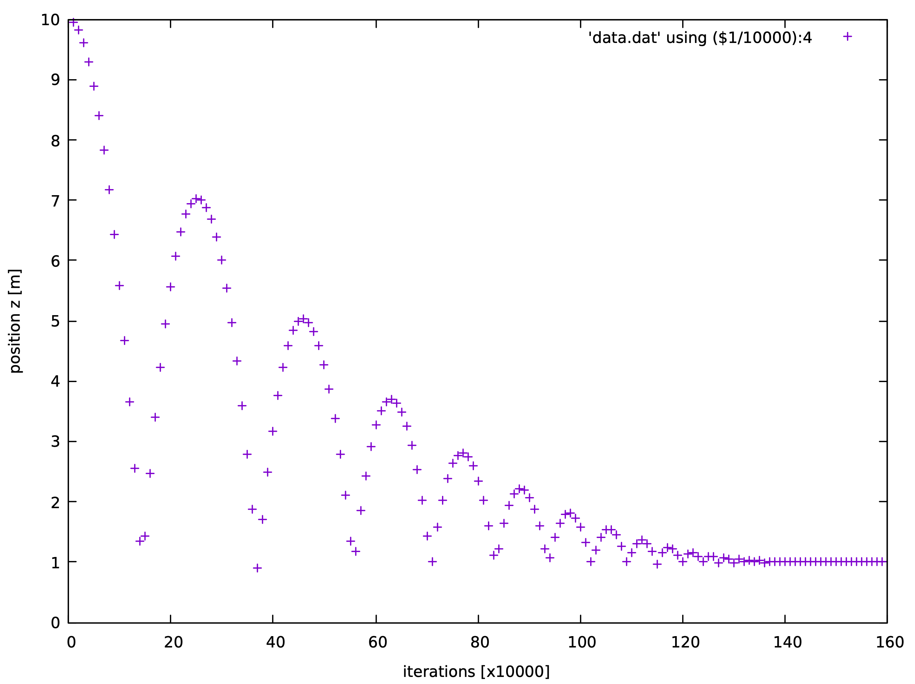
球体自由落体到地面的z方向坐标变化。
2.2 - 示例 1: 超级椭球堆积模拟
超级椭球局部坐标下的形状函数可由下式给出 $$\label{eqsurface} \Big(\big|\frac{x}{r_x}\big|^{\frac{2}{\epsilon_1}} + \big|\frac{y}{r_y}\big|^{\frac{2}{\epsilon_1}}\Big)^{\frac{\epsilon_1}{\epsilon_2}} + \big|\frac{z}{r_z}\big|^{\frac{2}{\epsilon_2}} = 1$$ 其中 $r_x, r_y$ 和 $r_z$ 是超级椭球在x, y, z轴的半长主轴; and $\epsilon_i (i=1,2)$ 是刻画颗粒棱角度的形状参数. $\epsilon_i$ 在 0 到 2 的变化可勾勒出非常丰富的凸超级椭球形状。SudoDEM 生成超级椭球的两个函数可参见如下高亮描述 (see Sec. 5.1.2{reference-type=“ref” reference=“modsuperquadrics”}):
-
NewSuperquadrics2($r_x$, $r_y$, $r_z$, $\epsilon_1$, $\epsilon_2$, mat, rotate, isSphere)
-
NewSuperquadrics_rot2($r_x$, $r_y$, $r_z$, $\epsilon_1$, $\epsilon_2$, mat, $q_w$, $q_x$, $q_y$, $q_z$, isSphere)
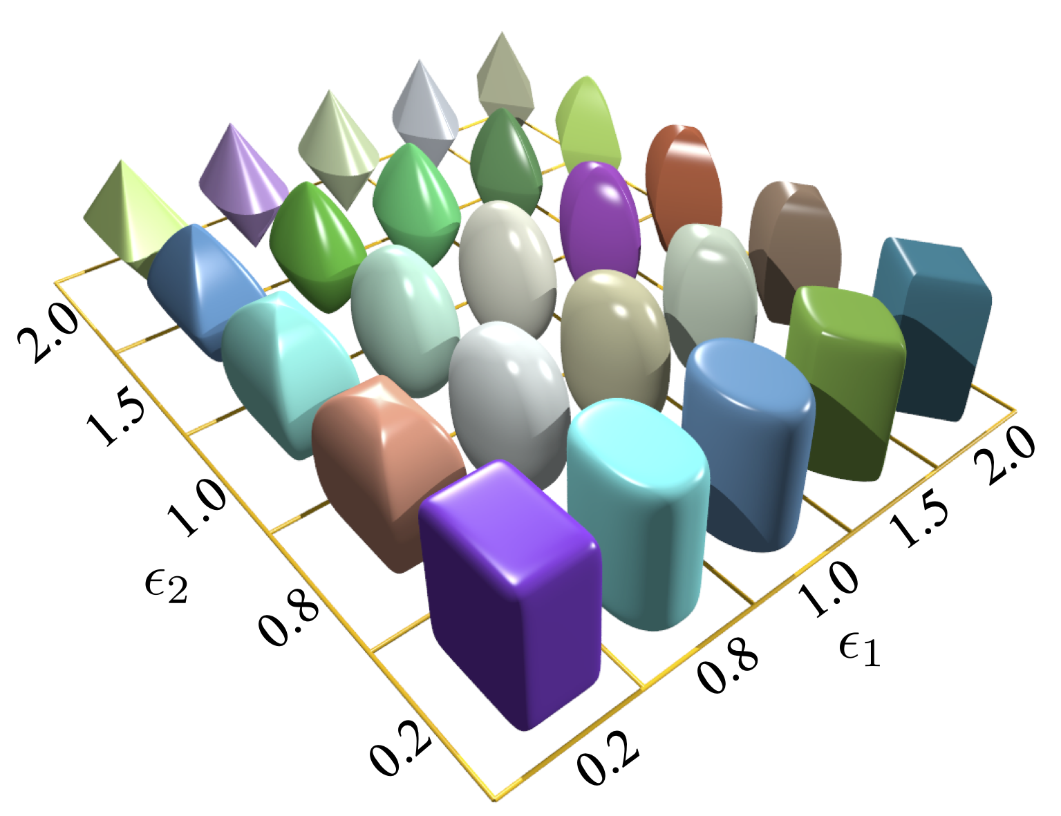
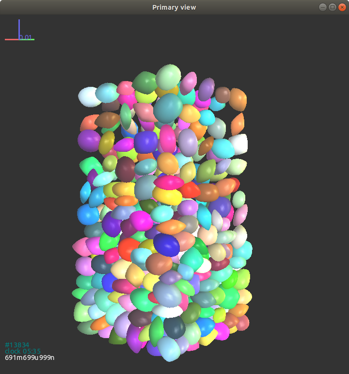
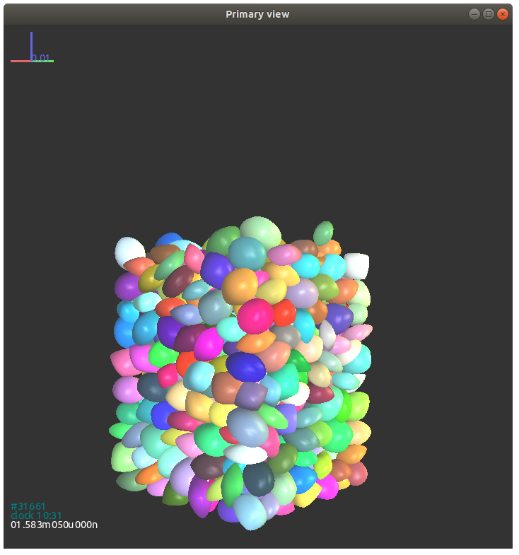
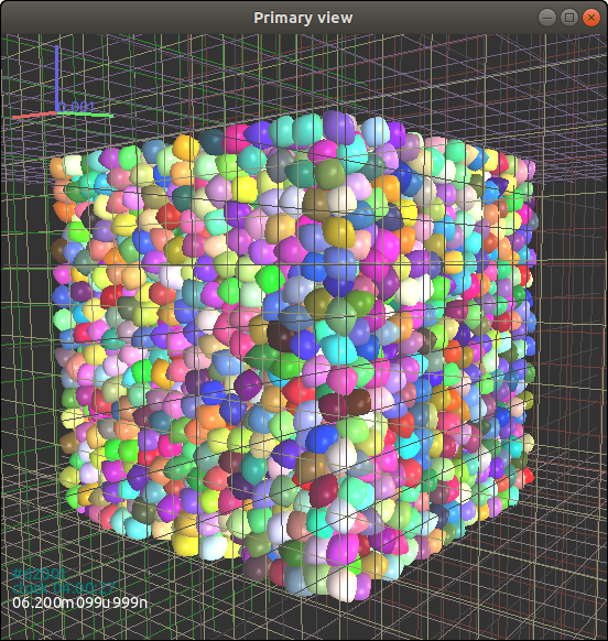
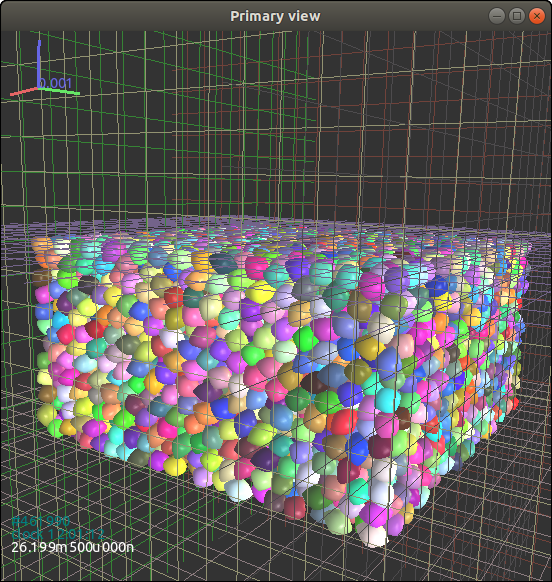
超级椭球。
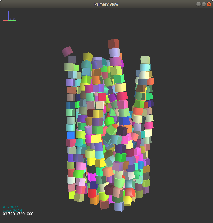
这里我们给出了超级椭球在立方体盒子中重力堆积的模拟示例。
|
|
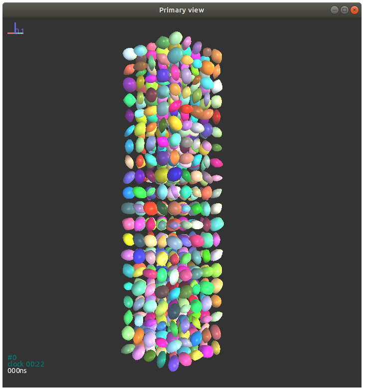
在GUI控制面板中我们可以通过点击 ‘show 3D’ 按钮来显示模拟的可视化场景。在显示模式下选择 ‘Gl1_Superquadrics’ 渲染器来控制颗粒是由线条还是由实体面来渲染(如图), 3.3{reference-type=“ref” reference=“figguidisplay”}.
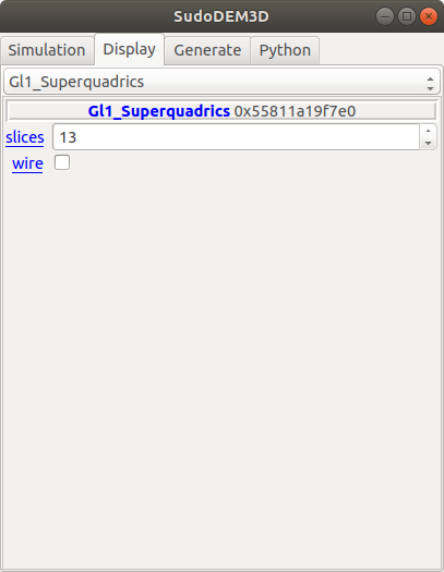
Figs. 3.4{reference-type=“ref” reference=“figexp11”} - 3.6{reference-type=“ref” reference=“figexp13”} 显示了在不同渲染模式下的超级椭球颗粒。
超级椭球颗粒的属性和类方法展示如下:
-
属性:
-
$r_x$, $r_y$, $r_z$: 浮点型, x, y, 和 z 轴的半长轴。
-
$\epsilon_1$, $\epsilon_2$: 浮点型, 材料参数。
-
isSphere: 布尔值, 颗粒是否是球体.
-
-
类方法:
-
getVolume(): 浮点型, 返回颗粒体积。
-
getrxyz(): 三阶向量, 返回颗粒的三个半长轴。
-
geteps(): 二阶向量, 返回颗粒的形状参数eps1和eps2。
-
如下代码给出了获取索引为100的超级椭球的体积:
volume = O.bodies[100].shape.getVolume()
获取对象所有属性的方法如下:
O.bodies[100].dict()
输出如下:
{'bound': <Aabb instance at 0x56072ec83da0>,
 'chain': -1,
 'clumpId': -1,
 'flags': 3,
 'groupMask': 1,
 'id': 100,
 'iterBorn': 0,
 'material': <SuperquadricsMat instance at 0x56072e6ed5f0>,
 'shape': <Superquadrics instance at 0x56072ec83b60>,
 'state': <State instance at 0x56072ec839e0>,
 'timeBorn': 0.0}
我们可以看到对象的属性是以字典的方式被打印出来的。需要提及的是尖括号内的是另一个对象的指针,也就是说我们可以通过dict()方法来进一步获取其对应的属性。例如我们要获取颗粒state的属性,可以通过如下代码:
O.bodies[100].state.dict()
输出如下:
{'angMom': Vector3(0,0,0),
 'angVel': Vector3(0,0,0),
 'blockedDOFs': 0,
 'densityScaling': 1.0,
 'inertia': Vector3(0.0045389863901528615,0.007287422614611933,
                           0.0067053718092146865),
 'isDamped': True,
 'mass': 3.225715855242557,
 'refOri': Quaternion((1,0,0),0),
 'refPos': Vector3(0,0,0),
 'se3': (Vector3(0,0.8,3),
  Quaternion((0.3970010520699211,0.5339678220536823,
                     -0.7465042060609055),2.1754719537556495)),
 'vel': Vector3(0,0,0)}
对于 Shape对象, 它的属性输出可能随着子类的不同而不同。
O.bodies[100].shape.dict()
输出如下:
{'color': Vector3(0.6407663308273844,0.07426042997942327,
                            0.05872324344642611),
 'eps': Vector2(1.3975848801318045,1.5376309088540607),
 'eps1': 1.3975848801318045,
 'eps2': 1.5376309088540607,
 'highlight': False,
 'isSphere': False,
 'rx': 0.1,
 'rxyz': Vector3(0.1,0.06469580193313924,0.07572423080016706),
 'ry': 0.06469580193313924,
 'rz': 0.07572423080016706,
 'wire': False}
这里我们给出了一个例子用来获取所有超级椭球的序号及其位置信息:
for b in O.bodies: # loop all bodies in the simulation
    # we have to check if the present body is a superellipsoid or others, e.g., a wall
    if isinstance(b.shape, Superquadrics): # if it is a superellipsoid, then to do
        pid = b.id # get the id of particle b
        pos = b.state.pos # get the position of particle b
        print pid, pos
2.3 - 示例 2: 超级椭球三轴试验模拟
该例子给出了超级椭球的三轴固结及压缩试验模拟。该模拟使用 CompressionEngine 引擎来完成, 同时用户可通过 PyRunner 引擎来自定义 CompressionEngine 引擎。固结和压缩引擎的基本设置如下:
-
固结
1 2 3 4 5 6 7 8 9 10 11 12 13 14 15triax=CompressionEngine( goalx = 1.0e5, # 围压 100 kPa goaly = 1.0e5, goalz = 1.0e5, savedata_interval = 10000, echo_interval = 2000, continueFlag = False, max_vel = 100.0, gain_alpha = 0.5, f_threshold = 0.01, fmin_threshold = 0.01, #偏应力与平均应力的比值 unbf_tol = 0.01, #不平衡力比值 file='record-con' )-
goalx = goaly = goalz = 围压
-
savedata_interval: 保存模拟信息 (轴应变,体应变,平均应力和偏应力) 到文件的DEM时步周期,在固结引擎中该选项已被弃用。
-
echo_interval: 显示模拟信息 (时步, 不平衡力比值, 各个方向的应力) 到命令行的DEM时步周期。
-
continueFlag: 用来表示继续固结或压缩的保留关键字。
-
max_vel: 墙体最大移动速度,可在固结时用于限制墙体的移动。
-
gain_alpha $\alpha$: 用来控制墙体下一步的移动速度。 $$v_w = \alpha \frac{f_w - f_g}{\Delta t \sum k_n}$$ 其中, $v_w$ 表示墙体在下一时步的移动速度; $f_w$ 和 $f_g$ 分别表示当前和目标接触力; $\Delta t$ 表示时步; $\sum k_n$ 表示墙体和所有接触颗粒的接触刚度之和。
-
f_threshold $\alpha_f$: 归一化的接触力偏离比值, 即, $$\alpha_f = \frac{|f_w-f_g|}{f_g}$$
-
fmin_threshold $\beta_f$: 偏应力 $q$ 和平均主应力 $p$ 的比值, 即, $$\beta_f = \frac{q}{p},\quad p= \frac{\sigma_{ii}}{3},\quad q=\sqrt{\frac{3}{2}\sigma_{ij}^{'}\sigma_{ij}^{'}}$$ $$\sigma_{ij} = \frac{1}{V}\sum_{c\in V}f_i^cl_j^c,\quad \sigma_{ij}^{'}=\sigma_{ij}-p\delta_{ij}$$ 其中 $\sigma_{ij}$ 表示颗粒集合体的应力张量, $\sigma_{ij}^{'}$ 表示应力张量的偏应力部分; $V$ 表示试样体积; $f^c$ 和 $l^c$ 分别表示接触 $c$ 的接触力和接触支向量; $\delta_{ij}$ 表示克罗纳克尔。
-
unbf_tol $\gamma_f$: 表示不平衡力比值,由下式给出 $$\gamma_f = \frac{\sum\limits_{B_i\in V} |\sum\limits_{j\in B_i}f^c_j+f^b_j|}{2\sum\limits_{c\in V}|f^c|}$$ 需要说明的是只有当 $\alpha_f$, $\beta_f$ 和 $\gamma_f$ 都达到设定值,固结过程才会结束。
-
file: 模拟信息输出的文件相关信息
-
-
压缩
1 2 3 4 5 6 7 8 9 10 11 12 13 14 15 16triax=CompressionEngine( z_servo = False, goalx = 1.0e5, goaly = 1.0e5, goalz = 0.01, ramp_interval = 10, ramp_chunks = 2, savedata_interval = 1000, echo_interval = 2000, max_vel = 10.0, gain_alpha = 0.5, file='sheardata', target_strain = 0.4, gain_alpha = 0.5 )-
z_servo: 布尔值,用来控制z方向是应变加载还是应力加载,在应变加载状态下 goalz 是对应的应变加载速率。
-
ramp_interval: 逐级加载到稳定应变速率的时步。该变量用来模拟实际试验中逐级稳定加载的过程,用户可以通过设定一个很小的值来忽略这个变量的影响。
-
ramp_chunks: 逐级加载到稳定应变速率的区间数。与 ramp_interval 类似,用户可以通过设定较小值来忽略它的影响。
-
target_strain: 加载目标应变 (对数应变),在应变达到该值的时候剪切模拟停止。
注: 如果用户需要进行准静态的三轴剪切模拟,剪切速率要低于一定的阈值。特别地,我们使用加载惯性系数来表征加载的准静态性, 即当惯性系数 $I$ 低于 $10^{-3}$时可视为准静态剪切,其中惯性系数由下式给出 $$I = \dot{\epsilon_1}\frac{\hat{d}}{\sqrt{\sigma_0/\rho}}$$ 其中 $\dot{\epsilon_1}=\mathrm{d}\epsilon_1/\mathrm{d}t$ 表示剪切应变加载速率; $\hat{d}$ 和 $\rho$ 分别表示颗粒的平均直径和平均密度, $\sigma_0$ 表示围压。
-
我们这里给出了一个三轴剪切加载的例子作为参考:
|
|
命令行将会有如下信息显示
calm procedure is over
0 particles are deleted!
consolidation begins
Iter 50000 Ubf 0.483161, Ss_x:9.67986e-05, Ss_y:4.15364e-05, Ss_z:6.1184e-05, e:0.992618
Iter 52000 Ubf 0.461741, Ss_x:1.2412, Ss_y:1.06812, Ss_z:1.10116, e:0.854445
Iter 54000 Ubf 0.263699, Ss_x:1.75334, Ss_y:1.98567, Ss_z:1.62181, e:0.757469
Iter 56000 Ubf 0.118329, Ss_x:3.06302, Ss_y:3.54818, Ss_z:3.22986, e:0.679106
Iter 58000 Ubf 0.0110747, Ss_x:22.0177, Ss_y:21.3303, Ss_z:21.3485, e:0.614824
Iter 60000 Ubf 0.000577066, Ss_x:91.4199, Ss_y:89.6039, Ss_z:89.1057, e:0.58984
Iter 62000 Ubf 0.000128293, Ss_x:100.012, Ss_y:99.7251, Ss_z:99.6123, e:0.587807
consolidation completed!
固结完成后 (如图 Fig. [3.7] 所示,(#figex2consol){reference-type=“ref” reference=“figex2consol”}), 我们可以保存固结完成后的颗粒状态到文件中
|
|
然后我们开始对固结后的试样进行剪切,参见下面的脚本:
|
|
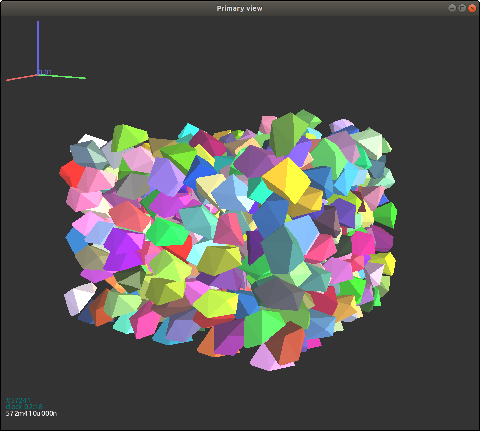
试样的剪切加载总应变为40%,剪切终止时的试样状态如图所示 Fig. 3.8{reference-type=“ref” reference=“figex2shear”}.
试样在剪切阶段的宏观力学响应可以用应力张量来表征,该张量由下式子得到: $$\label{eqDEMstress} \sigma_{ij} = \frac{1}{V} \sum_{c \in V} f_i^c l_j^c$$ 其中 $V$ 表示试样总体积; $f^c$ 表示接触 $c$ 的接触力矢量; $l^c$ 表示接触对应的支向量,也就是连接接触两颗粒质心的矢量。 平均主应力 $p$ 和偏应力 $q$ 被定义为: $$p = \frac{1}{3}\sigma_{ii},\quad q = \sqrt{\frac{3}{2} \sigma_{ij}^{'}\sigma_{ij}^{'}}$$ 其中 $\sigma_{ij}^{'}$ 表示应力张量的偏应力部分 $\sigma_{ij}$.
考虑到立方体试样的加载是由六个刚性墙来伺服控制的,轴向应变 $\epsilon_z$ 和 体应变 $\epsilon_v$ 可以由墙体的位置近似的给出, 即, $$\epsilon_z = \int_{H_0}^{H}\frac{\mathrm{d}h}{h}=-\ln\frac{H_0}{H},\quad \epsilon_v = \epsilon_x+\epsilon_y+\epsilon_z=\int_{V_0}^{V}\frac{\mathrm{d}v}{v}=-\ln\frac{V_0}{V}$$ 其中 $H$ 和 $V$ 分别表示剪切状态下的墙体高度和体积, $H_0$ 和 $V_0$ 表示刚性强初始状态的高度和体积。 体应变正值表示试样的剪胀状态。
剪切过程的数据保存格式如下:
AxialStrain VolStrain meanStress deviatorStress
0.000511000266 0.000490480823 106090.98 15931.56
0.003011001516 0.002450117535 131061.41 85718.91
0.005511002766 0.003867756447 148076.65 131980.95
0.008011004016 0.004825115794 159924.28 163706.90
0.010511005266 0.005409561745 168606.27 186520.14
0.013011006516 0.005673777079 175131.53 203243.28
0.015511007766 0.005650846281 180293.19 216248.17
0.018011009016 0.005393122254 184581.23 227010.23
进而我们可以绘制出三轴剪切过程的应力-应变曲线以及应力路径曲线,如图所示 Figs. 3.9{reference-type=“ref” reference=“figex2shearstress”} and 3.10{reference-type=“ref” reference=“figex2shearpath”}.
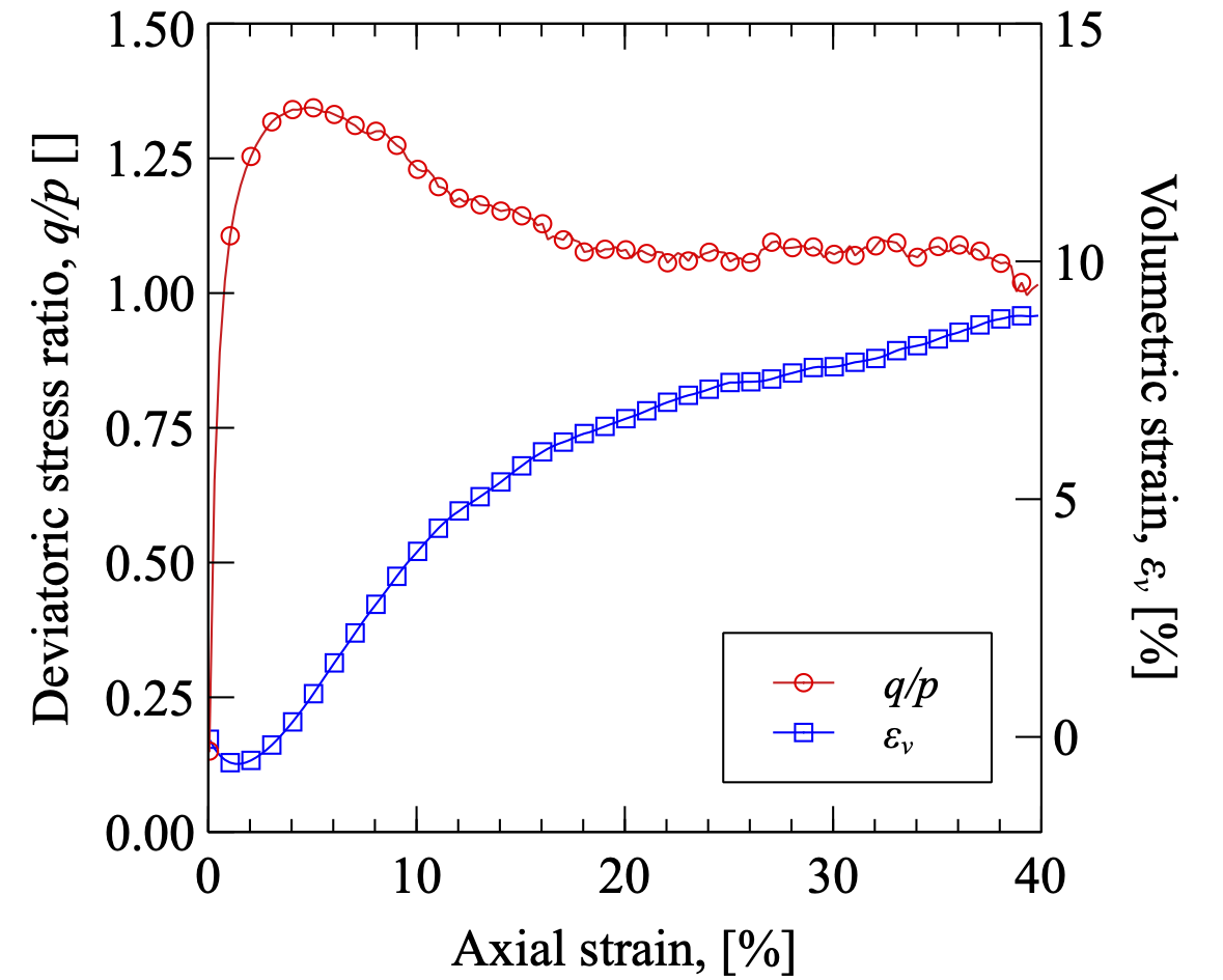
剪切过程中的应力应变曲线以及体应变曲线。
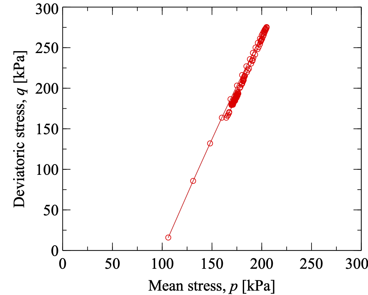
剪切过程中的应力路径变化。
在剪切过程中,试样状态会不断地被保存在文件中,(例如, "shearxxx.xml.bz2") 用于随后的后处理,比如我们可以利用试样加载的元数据来获得试样的配位数和组构等信息。
2.4 - 示例 3: GJK颗粒的堆积模拟
SudoDEM 中有五种颗粒它们的接触检测算法是用GJK算法实现的,即球体,多面体,圆锥体,圆柱体以及立方体[^5], 我们我们采用GJK颗粒来统一的归类如上颗粒。对应的,Python脚本中该颗粒可以用以下包来导入 _gjkparticle_utils (see Sec. 5.1.3{reference-type=“ref” reference=“modgjkparticle”}), 这五种颗粒的构造函数如下所示:
-
GJKSphere(radius,margin,mat)
-
GJKPolyhedron(vertices,extent,margin,mat, rotate)
-
GJKCone(radius, height, margin, mat, rotate)
-
GJKCylinder(radius, height, margin, mat, rotate)
-
GJKCuboid(extent, margin,mat, rotate)
注: 每个颗粒都被放大了一定的倍数用于加速颗粒接触检测算法,该放大倍数要足够大用以保证颗粒颗粒在较小尺度下可以发生接触, 同时该放大倍数要足够小,以避免颗粒形状的过度失真。
与示例1类似, 我们将会模拟GJK颗粒在立方体盒子中的自由落体堆积过程。进行模拟前,我们需要先导入如下包:
|
|
定义生成颗粒的参数信息:
|
|
定义颗粒生成栅格:
|
|
设置材料属性
|
|
生成立方体盒子
|
|
生成模拟引擎并设置固定时步:
|
|
多面体颗粒生成如下所示:
|
|
 {#figgjkpolyhedron width=“8cm”}
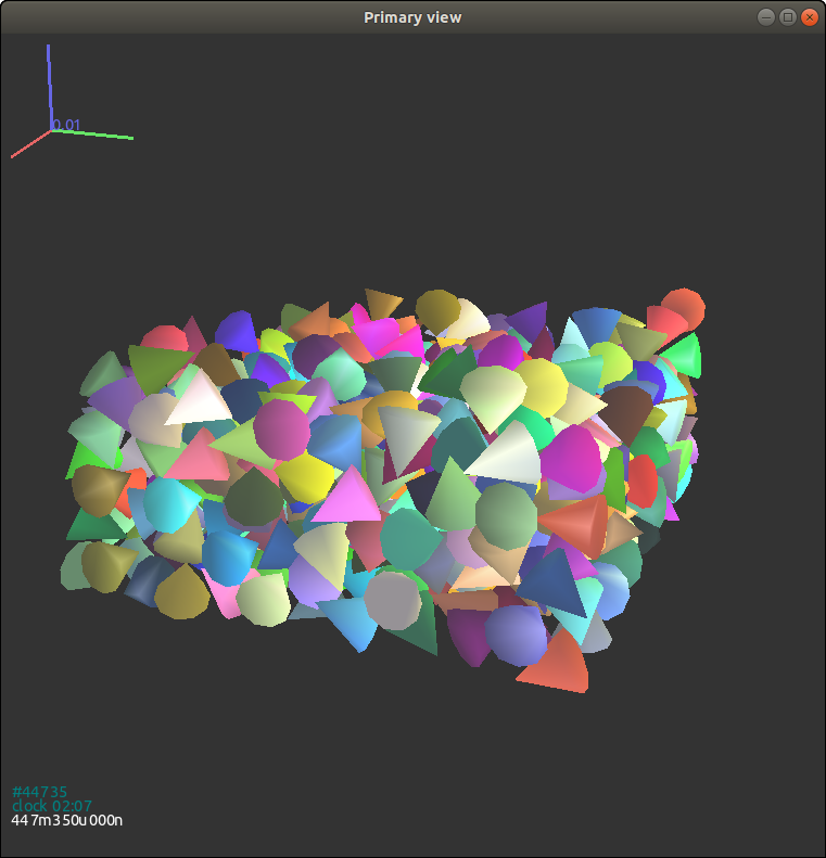
 {#figgjkcone width=“8cm”}
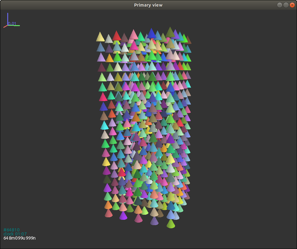
对于圆锥体来说函数 GenSample 需做如下改动:
|
|
Fig. 3.12{reference-type=“ref” reference=“figgjkcone”} 给出了固定初始朝向的圆锥体试样 (通过将变量 rotate 设置为 False 来取消随机的初始朝向生成)。 可以看到所有颗粒的初始状态都是完全相同的。
用户可以尝试将变量 rotate 设置为 True 来测试下随机初始朝向的颗粒试样:
|
|
 {#figgjkcone2 width=“8cm”}
如图所示,自由落体过程破坏了颗粒非常一致的初始朝向分布: 3.13{reference-type=“ref” reference=“figgjkcone2”}
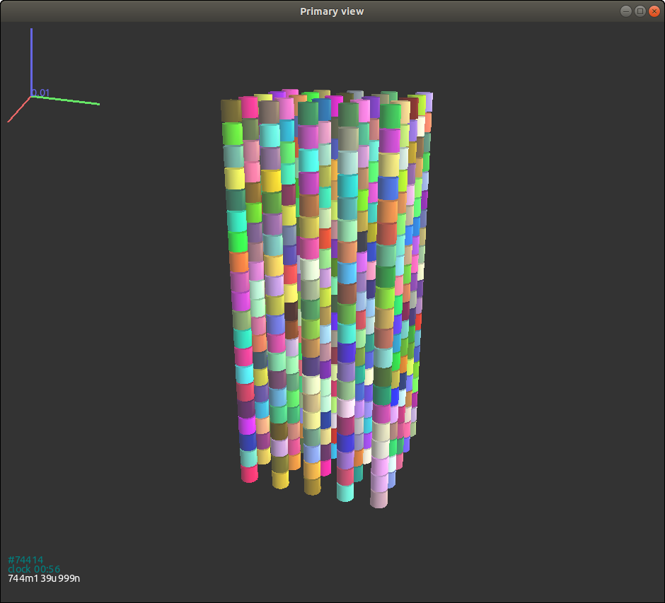 {#figgjkcylinder width=“8cm”}
圆柱的生成函数 GenSample 改动如下:
|
|
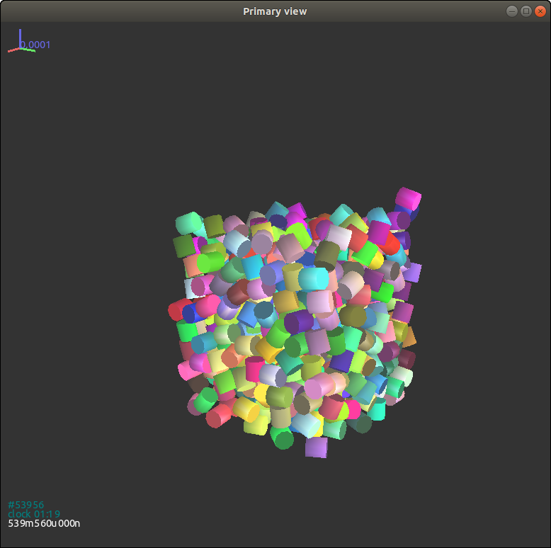 {#figgjkcylinder2 width=“8cm”}
不出意料,对于初始朝向一致的圆柱颗粒,即使是在自由落体后,它们的朝向仍然不变 Fig. 3.14{reference-type=“ref” reference=“figgjkcylinder”}。但是当初始朝向是随机生成时,自由落体结束后的圆柱体朝向变得不规律起来 3.15{reference-type=“ref” reference=“figgjkcylinder2”}。
|
|
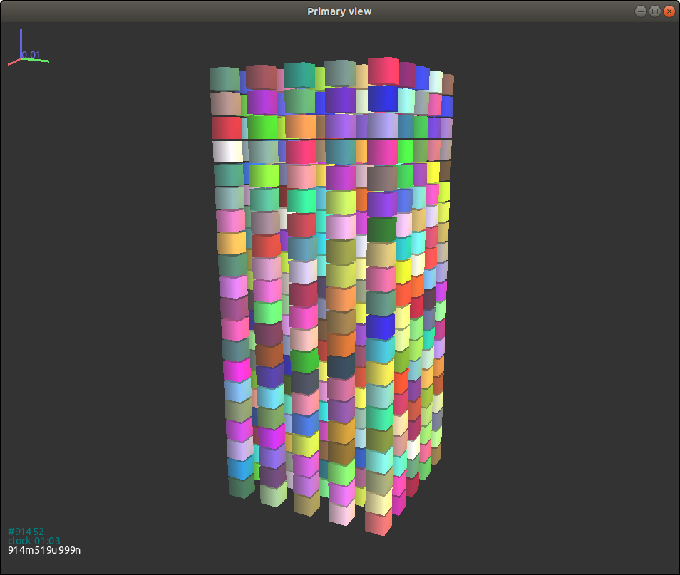 {#figgjkcuboid width=“8cm”}
 {#figgjkcuboid2 width=“8cm”}
立方体的函数如下:
|
|
立方体的初始一致或随机生成朝向的自由落体过程与圆柱体非常相似。在初始朝向一致时,如图所示Fig. 3.16{reference-type=“ref” reference=“figgjkcuboid”} 自由落体结束后朝向并未发生显著变化。 但是随机初始朝向的试样,在自由落体过程前后的朝向分布有巨大的差异。 True as follows:
|
|
另外,考虑到立方体颗粒间的间隙较小,所以它们的随机朝向在自由落体前后的分布差异较圆柱体不明显。
2.5 - 示例 4: 组合超级椭球的堆积模拟
组合超级椭球有形如真实颗粒(砂土)的如下显著的特性 (例如, 平直度,非对称性以及棱角度)。 组合超级椭球的形状函数可以通过组装八个超级椭球的形状参数得到: $$\Big(\big|\frac{x}{r_{x}}\big|^{\frac{2}{\epsilon_{1}}} + \big|\frac{y}{r_{y}}\big|^{\frac{2}{\epsilon_{1}}}\Big)^{\frac{\epsilon_{1}}{\epsilon_{2}}} +\big |\frac{z}{r_{z}}\big|^{\frac{2}{\epsilon_{2}}} = 1$$
::: {.subequations} $$\begin{aligned} r_{x} = r_x^+ \quad{}\text{if}\quad{} x\geq 0 \quad{}\text{else}\quad{} r_x^- \label{appa} \ r_{y} = r_y^+ \quad{}\text{if}\quad{} y\geq 0 \quad{}\text{else}\quad{} r_y^- \label{appb} \ r_{z} = r_z^+ \quad{}\text{if}\quad{} z\geq 0 \quad{}\text{else}\quad{} r_z^- \label{appc}\end{aligned}$$ :::
其中 $r_x^+,r_y^+,r_z^+$ 和 $r_x^-,r_y^-,r_z^-$ 分别表示颗粒在正负主轴 x, y, z 的长度; $\epsilon_1, \epsilon_2$ 控制颗粒表面的棱角度, 对于凸颗粒来说,它们取值范围在 $(0,2)$。 图 Fig. 3.18{reference-type=“ref” reference=“figmultipolysuper”} 形象的描述了 $\epsilon_1$ 和 $\epsilon_2$ 是如何影响颗粒形状的。 Python包 _superquadrics_utils 提供了两个用来生成组合超级椭球的函数 (参见 Sec. 5.1.2{reference-type=“ref” reference=“modsuperquadrics”}):
-
NewPolySuperellipsoid(eps, rxyz, mat, rotate, isSphere, inertiaScale = 1.0)
-
NewPolySuperellipsoid_rot(eps, rxyz, mat, $q_w$, $q_x$, $q_y$, $q_z$, isSphere, inertiaScale = 1.0)
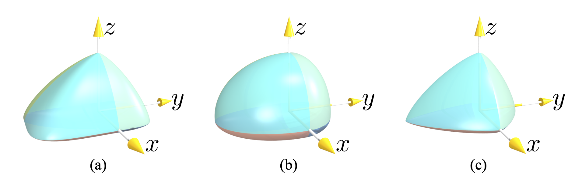 组合超级椭球及其形状参数
$r_x^+=1.0, r_x^-=0.5, r_y^+=0.8, r_y^- = 0.9, r_z^+ = 0.4, r_z^- = 0.6$
(a) $\epsilon_1=0.4, \epsilon_2=1.5$, (b)
$\epsilon_1=\epsilon_2=1.0$, (c)
$\epsilon_1=\epsilon_2=1.5$.
组合超级椭球及其形状参数
$r_x^+=1.0, r_x^-=0.5, r_y^+=0.8, r_y^- = 0.9, r_z^+ = 0.4, r_z^- = 0.6$
(a) $\epsilon_1=0.4, \epsilon_2=1.5$, (b)
$\epsilon_1=\epsilon_2=1.0$, (c)
$\epsilon_1=\epsilon_2=1.5$.
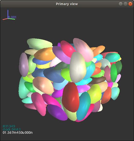
这里我们给出了组合超级椭球堆积模拟的示例脚本:
|
|
图 3.19{reference-type=“ref” reference=“figpolysuperpacking”} 给出了组合超级椭球堆积模拟的结果示意图。
 {#figpolysuperpacking
width=“10cm”}
{#figpolysuperpacking
width=“10cm”}
2.6 - 示例 5: 超椭圆堆积模拟
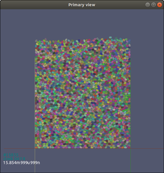
超椭圆局部坐标系下的形状函数如下式: $$\big|\frac{x}{r_x}\big|^{\frac{2}{\epsilon}} + \big|\frac{y}{r_y}\big|^{\frac{2}{\epsilon}} = 1$$ 其中 $r_x$ 和 $r_y$ 分别表示x和y轴的半长轴长度; $\epsilon \in (0, 2)$ 控制了颗粒表面的棱角度。 我们这里给出了超椭圆在重力作用下自由落体堆积的模拟脚本:
|
|
如上脚本需使用 sudodem2d 运行,模拟结果如图所示 Fig. 3.20{reference-type=“ref” reference=“figpackingellipse”}。
 {#figpackingellipse width=“10cm”}
3 - 后处理
数据
用户可以使用PyRunner引擎来保存 SudoDEM 运行中的数据:
|
|
Python 包 utilspost 提供了一系列的后处理函数用来协助用户后处理,包括应力-力-组构计算以及用于调用其他后处理软件的接口函数 (例如,颗粒形状的vtk文件保存函数, 颗粒信息3D直方图的vtk文件保存函数)。基于如上包用户可以非常容易调用或自定义适合自己的后处理函数。
|
|
Python 包 _superquadrics_utils 提供如下后处理辅助函数,
-
outputParticles(filename) : 该函数接收一个文件名,并将保存每个颗粒的形状信息到该文件中,包括形状参数 $r_x$, $r_y$, $r_z$, $\epsilon_1$, $\epsilon_2$, 位置 $x$, $y$, $z$, 和朝向 $q0$,$q1$,$q2$,$q3$ (等价于 $q_w$, $q_x$, $q_y$, $q_z$)。
-
outputParticlesbyIds(filename, ids) : 该函数接收一个文件名以及颗粒索引,该函数将具有该索引的颗粒的信息保存到该文件中,保存信息与 outputParticles(filename) 相同。
-
outputWalls(filename) : 该函数接收一个文件名, 并将墙体的位置信息保存到该文件中。
-
outputPOV(filename) : 该函数接收一个文件名,并将颗粒的信息以POV-Ray文件格式保存,该POV-Ray文件可被用于POV-Ray进行颗粒的渲染。
-
outputVTK(filename,slices) : 该函数接收一个文件名,并将颗粒的信息以VTK文件格式保存,用户可以使用Paraview等VTK软件对颗粒进行渲染。
颗粒模拟可视化
SudoDEM3D
我们强烈推荐两款开源且免费的可视化软件用于 SudoDEM 的后处理可视化 Paraview[^6] and POV-Ray[^7]:
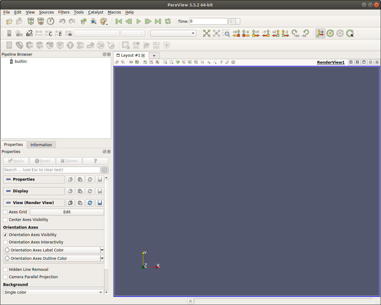 {#figparaview width=“10cm”}
高精度的颗粒信息可视化相较于简单的截图可以更清晰表征模拟结果。这里我们将为大家演示如何利用vtk或者pov文件进行高精度颗粒信息可视化, 我们假设计算结果已经被保存至文件 "shearend.xml.bz2" 。
|
|
打开 Paraview, 导入vtk文件 "shearend.vtk" 然后点击按钮 "Apply" 从而得到如下图所示的可视化结果 Fig. 4.2{reference-type=“ref” reference=“figshearendvtk”}。 需要说明的是函数 outputVTK 将颗粒的表面视为多面体的切片组合 (切片的精度这里被设置为 15) , 依此法可能会得到较大的后处理文件 (该例子文件大约180 Mb)。 基于此用户可以选择多种多样的方式来减少后处理文件大小,比如用户可以通过 Paraview 提供的快速可视化方法,或者 可以利用 Paraview 内置接口 Superquadric 来降低可视化文件大小。
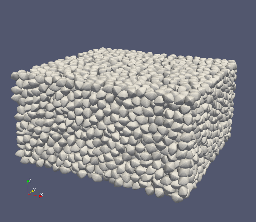 {#figshearendvtk width=“8cm”}
用户还可以通过使用POV-Ray 来降低可视化文件大小。
|
|
用户可以通过修改POV文件的相机设置来达到自定义的可视化效果, i.e., "shearend.pov" here,
|
|
这里给出了如何自定义光源的设置。
|
|
在命令行中运行如下命令来可视化颗粒:
povray shearend.pov
如果要修改可视化精度,用户可以添加额外的命令参数来达到这一目的,
povray shearend.pov +A0.01 +W1600 +H1200
图像处理软件, 例如, GIMP [^8], 可用来修改图片大小或者制作动图。图 Fig. 4.3{reference-type=“ref” reference=“figshearend”} 给出了使用 POV-Ray 渲染并利用 GIMP 裁剪的颗粒渲染图片。
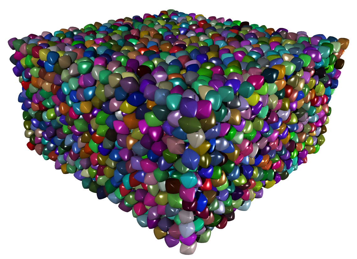 {#figshearend width=“8cm”}
包 snapshot 提供了组合超椭球的可视化函数。例如,我们导入堆积结果完成时的颗粒状态文件并利用 snapshot 进行POV文件生成:
|
|
此处我们得到两个文件分别是 packingpolysuper.inc 和 packingpolysuper.pov。 第一个文件 packingpolysuper.inc 包含了一些组合超椭球的宏定义以及颗粒形状参数信息,例如颗粒形状参数,颗粒位置,颗粒朝向等
|
|
我们不建议用户直接修改第一个文件,但是用户可以通过修改第二个文件来达到自定义渲染效果:
|
|
命令行输入以下命令来完成渲染
povray packingpolysuper.pov +A0.01 +W1600 +H1200
渲染完毕后用户将会得到如图所示的高精度后处理图片 Fig. 4.4{reference-type=“ref” reference=“figpolypov”}.
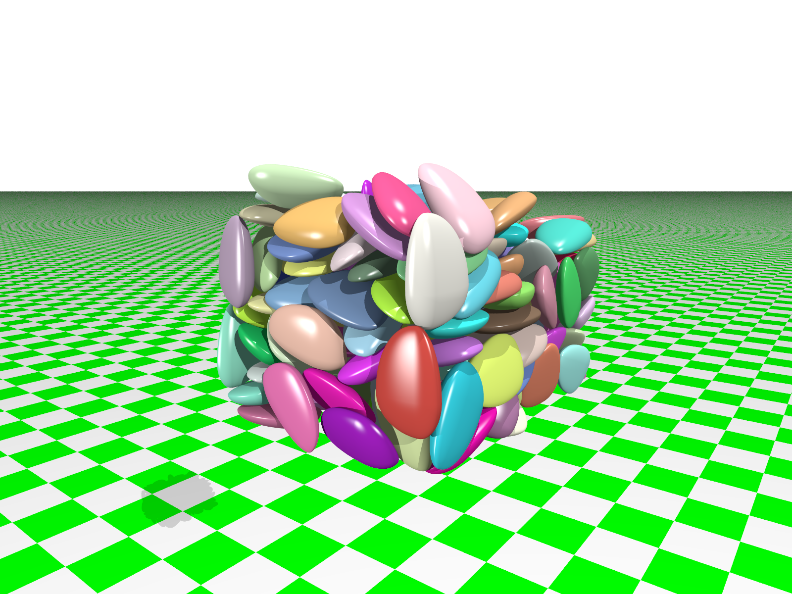 {#figpolypov width=“10cm”}
SudoDEM2D
包 _superellipse_utils 提供了名为 drawSVG (see Sec. 5.2.2{reference-type=“ref” reference=“secmodsuperellipse”}) 的函数用于绘制颗粒力链的矢量图。
|
|
生成的矢量图文件可以通过文本编辑器或者矢量图编辑器 Inkscape (推荐)来修改。图 Fig. 4.5{reference-type=“ref” reference=“figellipsesvg”} 给出了椭球颗粒在周期边界条件下堆积过程结束后的力链矢量图示例,用户可通过 drawSVG 函数来配置对应的输出图片格式。
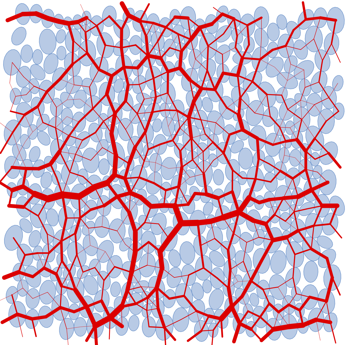 {#figellipsesvg width=“10cm”}
4 - Python类参考文档
SudoDEM3D
基类
class State(继承自 Serializable 类)
颗粒的状态 (空间位置,固有的物理状态)。
-
angMom(=Vector3r::Zero())
当前时步角动量 -
angVel(=Vector3r::Zero())
当前时步角速度 -
blockedDOFs
平动/转动的自由度约束状态。 该变量设置后,相应的平动或转动将保持在一个恒定值。 若要约束颗粒所有的平动及转动速度,可以使用字符串 ‘xyzXYZ’。 -
dict() → dict
返回状态的字典。 -
inertia(=Vector3r::Zero())
颗粒在局部坐标的转动惯量。 -
isDamped(=true)
该布尔值设置为false后颗粒在牛顿积分引擎中的计算将不考虑阻尼, 例如在模拟颗粒自由落体时,人工阻尼的引入将会导致错误的计算结果。 -
mass(=0)
颗粒的质量 -
ori
颗粒的旋转属性 -
pos
颗粒当前时步的位置 -
refOri(=Quaternionr::Identity())
颗粒参考旋转坐标 -
refPos(=Vector3r::Zero())
颗粒参考位置 -
se3(=Se3r(Vector3r::Zero(), Quaternionr::Identity()))
封装颗粒的位置和旋转坐标在一个变量中
超二次椭球模块 _superquadrics_utils
-
NewSuperquadrics2($r_x$, $r_y$, $r_z$, $\epsilon_1$, $\epsilon_2$, mat, rotate, isSphere)
该函数用于生成超二次椭球。-
$r_x$, $r_y$, $r_z$: float, 超二次椭球的半长轴
-
$\epsilon_1$, $\epsilon_2$: float, 超二次椭球形状参数
-
mat: Material, 超二次椭球的材料属性
-
rotate: bool, 超二次椭球在生成时是否被赋予随机旋转朝向
-
isSphere: bool, 超二次椭球是否是球体
-
-
NewSuperquadrics_rot2($r_x$, $r_y$, $r_z$, $\epsilon_1$, $\epsilon_2$, mat, $q_w$, $q_x$, $q_y$, $q_z$, isSphere)
该函数用于生成具备特定旋转朝向的超二次椭球。 $q_w$, $q_x$, $q_y$, $q_z$ 用于表征颗粒的旋转四元数,isSphere 用于决定颗粒是否为球体。-
$r_x$, $r_y$, $r_z$: float, 超二次椭球的半长轴
-
$\epsilon_1$, $\epsilon_2$: float, 超二次椭球形状参数
-
mat: Material, 超二次椭球的材料属性
-
isSphere: bool, 超二次椭球是否是球体
-
$q_w$, $q_x$, $q_y$, $q_z$: float, 颗粒的旋转四元数
-
-
outputWalls(filename)
输出当前模拟试样中的墙体位置- filename: string, 墙体位置保存文件的文件名
-
getSurfArea(id, w, h)
输出特定颗粒索引的表面积,该表面积由两个精度参数w 和 h 来控制,比如 w=10,h=10。 更大的 w 和 h值可以得到更高精度的表面积值。-
id: int, 颗粒索引
-
w, h: int, w$\times$h 将颗粒表面剖分为较小的四边形以此来进行表面积计算
-
-
outputParticles(filename)
输出所有颗粒信息到文件中,包括颗粒的索引,形状参数以及颗粒朝向信息到文件中- filename: string, 颗粒信息保存文件文件名
-
outputParticlesbyIds(filename, ids)
输出指定索引的颗粒信息到文件中,包括颗粒的索引,形状参数以及颗粒朝向信息到文件中 [Only for superellipsoids]-
filename: string, 颗粒信息保存文件文件名
-
ids: list of int, 颗粒索引列表, 例如, [10, 24, 22].
-
-
NewPolySuperellipsoid(eps, rxyz, mat, rotate, isSphere, inertiaScale = 1.0)
生成组合超二次椭球颗粒-
$eps$: Vector2, 组合超二次椭球的形状参数 即, [$\epsilon_1$, $\epsilon_2$].
-
$rxyz$: Vector6, 颗粒在三个正交坐标 (x, y, z) 的正向以及负向的半长轴, 即[$r_x^-$, $r_x^+$, $r_y^-$, $r_y^+$, $r_z^-$, $r_z^+$].
-
mat: Material, 组合超二次椭球的材料属性
-
rotate: bool, 生成的组合超二次椭球是否被赋予随机朝向
-
isSphere: bool, 生成的组合超二次椭球是否为球体
-
inertialScale: float, 用于缩放颗粒的转动惯量,如果尚未仔细了解此变量施加后的实际效果,请谨慎行事
-
-
NewPolySuperellipsoid_rot(eps, rxyz, mat, $q_w$, $q_x$, $q_y$, $q_z$, isSphere, inertiaScale = 1.0)
生成具有指定旋转属性的组合超二次椭球颗粒-
$eps$: Vector2, 组合超二次椭球的形状参数 即, [$\epsilon_1$, $\epsilon_2$].
-
$rxyz$: Vector6, 颗粒在三个正交坐标 (x, y, z) 的正向以及负向的半长轴, 即[$r_x^-$, $r_x^+$, $r_y^-$, $r_y^+$, $r_z^-$, $r_z^+$].
-
mat: Material, 组合超二次椭球的材料属性
-
isSphere: bool, 生成的组合超二次椭球是否为球体
-
$q_w$, $q_x$, $q_y$ and $q_z$: float, 组合超二次椭球的四元数参数 ($q_w$, $q_x$, $q_y$, $q_z$)
-
inertialScale: float, 用于缩放颗粒的转动惯量,如果尚未仔细了解此变量施加后的实际效果,请谨慎行事
-
-
outputPOV(filename)
输出超二次椭球(包括球体)的 POV 渲染信息到文本文件中,以便于用于可以使用 POV-ray来后处理相应的模拟结果 [目前仅支持超二次椭球以及球体]- filename: string, POV文件文件名
-
PolySuperellipsoidPOV(filename, ids = [], scale = 1.0)
输出组合超二次椭球的 POV 渲染信息到文本文件中,输出文件包括 *.inc 等文件, 用户可以通过修改该文件来改变相应的相机设置。详情请参见模块 snapshot.-
filename: string, POV文件文件名
-
ids: list of int, 给定的颗粒索引列表,若列表为空,则默认输出所有颗粒的信息。
-
scale: float, 用于对长度单位进行缩放。
-
-
outputVTK(filename, slices)
输出超二次椭球的颗粒信息到VTK文件中,以便于用户可以使用 Paraview 来对计算结果进行后处理。 [仅支持超二次椭球]-
filename: string, 输出文件的文件名
-
slices: int, 颗粒表面的离散精度
-
模块 _gjkparticle_utils
-
GJKSphere(radius,margin,mat)
-
radius, float, 球体半径
-
margin, float, 颗粒表面较小的边缘,用于辅助颗粒之间的接触检测
-
mat, Material, 颗粒材料属性
-
-
GJKPolyhedron(vertices,extent,margin,mat, rotate)
-
vertices, 多面体顶点列表,每个列表表征一个顶点的坐标, 例如, $[x, y, z]$。
-
extent, 用于缩放顶点的系数,尽在 vertices 为空时有效 (例如, $ $); 随机形状的多面体将基于Voronoi剖分生成。
-
margin, float, 颗粒表面较小的边缘,用于辅助颗粒之间的接触检测
-
mat, Material, 颗粒材料属性
-
rotate, bool, 颗粒是否在生成时被赋予随机旋转朝向
-
-
GJKCone(radius, height, margin, mat, rotate)
-
radius, float, 圆锥基地半径
-
height, float, 圆锥高
-
margin, float, 颗粒表面较小的边缘,用于辅助颗粒之间的接触检测
-
mat, Material, 颗粒材料属性
-
rotate, bool, 颗粒是否在生成时被赋予随机旋转朝向
-
-
GJKCylinder(radius, height, margin, mat, rotate)
-
radius, float, 圆柱半径
-
height, float, 圆柱高
-
margin, float, 颗粒表面较小的边缘,用于辅助颗粒之间的接触检测
-
mat, Material, 颗粒材料属性
-
rotate, bool, 颗粒是否在生成时被赋予随机旋转朝向
-
-
GJKCuboid(extent, margin,mat, rotate)
-
extent, 缩放系数用于缩放立方体在三维空间的尺寸
-
margin, float, 颗粒表面较小的边缘,用于辅助颗粒之间的接触检测
-
mat, Material, 颗粒材料属性
-
rotate, bool, 颗粒是否在生成时被赋予随机旋转朝向
-
注: 每个颗粒都被设置了一个较小的边缘尺寸用于加速颗粒的接触检测,该边缘应该足够大以满足颗粒接触检测的精度, 同时该边缘也应该足够小以至于不影响颗粒的实际形状尺寸。
模块 snapshot
-
outputBoxPov(filename, x, y, z, r=0.001, wallMask=[1,0,1,0,0,1])
输出立方体的 *.POV 文件 (x=[x_min, x_max], y=[y_min, y_max], z=[z_min, z_max]) 以便于用户使用 Pov-ray 进行后处理。-
filename: string, POV 文件名
-
x, y, z: Vector2, 立方体在三维空间的尺寸大小
-
r: float, 立方体盒子边缘大小
-
wallMask, list of 6 int, 该掩码用于设置六面墙体的消隐 (x-, x+, y-, y+, z-, z+)。 1 表示显示, 0 表示隐去。
-
-
outPov(fname,transmit=0,phong=1.0,singleColor=True,ids=[],scale=1.0, withbox = True)\
-
filename, string, POV 文件名
-
transmit, float, 颗粒的透明度大小,取值为0到1
-
phong, float, 颗粒亮度强光设置,取值为0到1
-
singleColor, bool, 是否为颗粒采用单一颜色,若否,则颗粒的颜色设置将视形状而定
-
ids, list of int, 指定的输出颗粒索引列表。若列表为空则默认输出所有颗粒信息。
-
scale, float, 缩放颗粒的长度尺寸
用户可参见 POV-Ray 相关手册来详细了解该函数所使用的 POV-Ray 内置变量的信息,例如 transmit 和 phong。
-
SudoDEM2D
基类
Class State
颗粒的状态 (空间位置,固有的物理状态)。
-
angMom(=Vector2r::Zero())
当前时步角动量 -
angVel(=Vector2r::Zero())
当前时步角速度 -
blockedDOFs
平动/转动的自由度约束状态。 该变量设置后,相应的平动或转动将保持在一个恒定值。 若要约束颗粒所有的平动及转动速度,可以使用字符串 ‘xyZ’。 -
dict() → dict
返回状态的字典。 -
inertia(=Vector2r::Zero())
颗粒在局部坐标的转动惯量。 -
isDamped(=true)
该布尔值设置为false后颗粒在牛顿积分引擎中的计算将不考虑阻尼, 例如在模拟颗粒自由落体时,人工阻尼的引入将会导致错误的计算结果。 -
mass(=0)
颗粒的质量 -
ori
颗粒的旋转属性,该旋转变量使用 Rotation2d 对象 (参见 Eigen 库 Rotation2D ), 该对象具有如下方法
Class Rotation2d-
angle: float, 用弧度制表征的旋转角度
-
toRotationMatrix(): Matrix2r, 返回响应的 2 $\times$ 2旋转矩阵
-
Identity(): Roation2d, 返回单位旋转矩阵
-
smallestAngle(): float, 返回旋转角度,取值为 $[-\pi,\pi]$
-
inverse(): Roation2d, 返回逆旋转状态
-
smallestPositiveAngle(): float, 返回旋转角度,取值为 $[0,2\pi]$
-
-
pos
颗粒当前时步的位置 -
refOri(=Rotation2D::Identity())
颗粒参考旋转坐标 -
refPos(=Vector2r::Zero())
颗粒参考位置 -
se2(=Se2r(Vector2r::Zero(), Rotation2d::Identity()))
封装颗粒的位置和旋转坐标在一个变量中 -
vel(=Vector2r::Zero()) 当前颗粒的平动速度
模块 _superellipse_utils
-
NewSuperellipse(rx, ry, epsilon, material, rotate, isSphere, z_dim =1.0)
该函数用于生成超二次椭圆。
-
rx, ry: float, 超二次椭圆的半长轴
-
epsilon: float, 超二次椭圆形状参数
-
material: 超二次椭圆的材料属性
-
rotate: bool, 超二次椭圆在生成时是否被赋予随机旋转朝向
-
isSphere: bool, 超二次椭圆是否是球体,该变量用于加速计算
-
z_dim: float, 颗粒在z方向的虚拟厚度,默认为1
-
-
NewSuperellipse_rot(x, y, epsilon, material, miniAngle, isSphere, z_dim = 1.0)
该函数用于生成具备特定旋转朝向的超二次椭圆
-
rx, ry: float, 超二次椭圆的半长轴
-
epsilon: float, 超二次椭圆形状参数
-
material: 超二次椭圆的材料属性
-
miniAngle: 颗粒的旋转四元数
-
isSphere: bool, 超二次椭圆是否是球体,该变量用于加速计算
-
z_dim: float, 颗粒在z方向的虚拟厚度,默认为1
-
-
outputParticles(filename)
输出所有颗粒信息到文件中,包括颗粒的索引,形状参数以及颗粒朝向信息到文本文件中
-
drawSVG(filename, width_cm = 10.0, slice = 20, line_width = 0.1, fill_opacity = 0.5, draw_filled = true, draw_lines = true, color_po = false, po_color = Vector3r(1.0,0.0,0.0), solo_color = Vector3r(0,0,0), force_line_width = 0.001, force_fill_opacity = 0, force_line_color = Vector3r(1.0,1.0,1.0), draw_forcechain = false)
输出颗粒的轮廓以及力链信息到 SVG 文件中
-
filename: string, 输出文件名
-
width_cm: float, SVG 头部信息中的宽度
-
slice: int, 超椭圆的剖分数量
-
line_width: float, 超椭圆边缘轮廓线的宽度
-
fill_opacity: float, 超椭圆填充颜色的透明度
-
draw_filled: bool, 超椭圆是否进行颜色填充
-
draw_lines: bool, 是否输出超椭圆的轮廓线
-
color_po: bool, 是否使用填充颜色来表征超椭圆的朝向
-
po_color: Vector3r, 用于表征超椭圆朝向的颜色 RGB
-
solo_color: Vector3r, 超椭圆填充颜色,若该值为0则使用 po_color 定义的颜色或使用 shape$\rightarrow$color
-
force_line_width: float, 力链线条的宽度
-
force_fill_opacity: float, 力链线条透明度
-
force_line_color: Vector3r, 力链线条颜色
-
draw_forcechain: bool, 是否将力链信息叠加绘制在颗粒轮廓上
-
模块 _utils
-
unbalancedForce(useMaxForce=false)
计算平均或最大不平衡力(若要计算最大不平衡力,使用 *useMaxForce*)。 For 对于绝对静止的平衡系统来说,所有颗粒的合力为0; 对于特定数值模拟, 理论上来说该不平衡力系数将随着模拟的进行渐趋于0,但是考虑到计算的精度问题,该不平衡力系数只能有限度的趋近于0。 用户可以设置足够小的不平衡力系数,例如1e-2或更小, 该值的具体设置取决于实际的模拟问题。
-
getParticleVolume2D()
模拟中颗粒的总体积 -
getMeanCN()
获取颗粒的平均配位数 -
changeParticleSize2D(alpha)
以特定比例来放大颗粒 -
getVoidRatio2D(cellArea=1)
计算颗粒试样的二维孔隙比,变量 cellArea 仅在非周期边界情况下适用 -
getStress2D(z_dim=1)
计算周期边界下试样的应力张量 -
getFabricTensorCN2D()
计算颗粒接触法向的组构张量 -
getFabricTensorPO2D()
计算颗粒朝向的组构张量 -
getStressAndTangent2D(z_dim=1,symmetry=true)
计算周期边界下的颗粒应力张量以及对应的雅克比: $S_{ijkl}=\frac{1}{V}\sum_{c}(k_n n_i l_j n_k l_l + k_t t_i l_j t_k l_l)$ -
getStressTangentThermal2D(z_dim=1, symmetry =true)
计算周期边界下考虑热应力耦合的颗粒应力张量以及对应的雅克比: $S_{ijkl}=\frac{1}{V}\sum_{c}(k_n n_i l_j n_k l_l + k_t t_i l_j t_k l_l)$
模块 utils
-
disk(center, radius, z_dim=1, dynamic=None, fixed=False, wire=False, color=None, highlight=False, material=-1,mask=1)
生成圆盘-
center: Vector2, 圆盘坐标
-
radius: float, 圆盘半径
-
dynamic: float, 已被弃用
-
fixed: float, 是否约束颗粒的自由度
-
material: 颗粒材料属性有如下定义方式
-
int: 颗粒将采用 O.materials[material] ; 若 material==-1 且对应颗粒材料无定义,utils.defaultMaterial() 将被设置为 O.materials[0]
-
string: 已存在的颗粒材料的标签
-
‘Material’ instance: 颗粒材料对象
-
callable: 无参调用; 返回颗粒材料值
-
-
int mask: 颗粒形状的掩码 ‘Body.mask’
-
wire: GUI显示中该颗粒将用线条而不是面来渲染
-
highlight: GUI中该颗粒是否高亮显示
-
Vector2-or-None: 颗粒颜色, 归一化的 RGB; 若该值定义为 None,则颗粒颜色为随机设置
-
-
wall(position, axis, sense=0, color=None, material=-1, mask=1)
返回墙体-
position: float-or-Vector3 , 墙体中心位置。若给定一维浮点数,则其他两个分量自动填充为0。
-
axis: {0,1} , 墙体的朝向
-
sense: {-1,0,1} , 激活墙体的接触检测,若设为0,则墙体的两侧接触检测都被激活,若设为-1,墙体仅在负方向激活接触检测;反之,反之
其他参数的具体定义请参见文档 ‘utils.disk’。
-
-
fwall(vertex1, vertex2, dynamic=None, fixed=True, color=None, highlight=False, noBound=False, material=-1, mask=1, chain=-1)
返回fwall墙体,该类与wall的区别在于,fwall是有限范围而wall是无限大范围-
vertex1: Vector2, 顶点1的全局坐标
-
vertex2: Vector2, 顶点2的全局坐标
-
noBound: bool, 设置对应的 ‘Body.bounded’
-
color: Vector3-or-None , fwall的颜色; 若改定为None则采用随机颜色
其他参数的具体定义请参见文档 ‘utils.disk’。
-