Post-processing

Data

It is preferable to save a series of states during a simulation, i.e., periodically saving data using a PyRunner:

1
2
3
4
5
6
7

def savedata():
        global saving_num
        saving_num += 1
        #print "testing, no data saved"
        O.save('shear'+str(saving_num)+'.xml.bz2')  
        
O.engines = O.engines + [PyRunner( command = 'savedata()', iterPeriod = 1000 )] # if we load the consolidation data, then we do not need this line because the PyRunner calling 'savedata()' has been defined.

The Python module utilspost provides plentiful examples of post-processing, including some basic functions of stress-force-fabric computation and other pre-processing functions for visualization (e.g., writing vtk files of particles and 3D histograms of fabric). Based on this module, users can copy and modify for a self purpose or just call the module functions in a post-processing script, e.g.,

1
2
3
4

import sudodem.utilspost as utilspost
#the following functions will output the average friction mobilization index of each state to a single file.
for i in ['1.0','1.2','1.4','1.6']:
    utilspost.calc_avgFricMobilIndex(i,steps_num)

The Python module _superquadrics_utils also provides some auxiliary functions, e.g.,

• outputParticles(filename) : filename, the file name for writing; output info of each particle, i.e., shape parameters $r_x$, $r_y$, $r_z$, $\epsilon_1$, $\epsilon_2$, position $x$, $y$, $z$, and orientation $q0$,$q1$,$q2$,$q3$ (equivalent to $q_w$, $q_x$, $q_y$, $q_z$ line by line. respectively).

• outputParticlesbyIds(filename, ids) : filename, the file name for writing; ids, a list of ids for particles needed outputting; output info of each particle in the list ids, i.e., shape parameters $r_x$, $r_y$, $r_z$, $\epsilon_1$, $\epsilon_2$, position $x$, $y$, $z$, and orientation $q0$,$q1$,$q2$,$q3$ (equivalent to $q_w$, $q_x$, $q_y$, $q_z$ line by line. respectively).

• outputWalls(filename) : filename, the file name for writing; output positions of all walls.

• outputPOV(filename) : filename, the file name for writing; output a POV-Ray file of particles for render using POV-Ray.

• outputVTK(filename,slices) : filename, the file name for writing; slices, number of slices a particle needed slicing in longitude; output a vtk file of particles for render using Paraview.

Scene Visualization

SudoDEM3D

For visualization, two free, open-source post-processing softwares, Paraview[^6] and POV-Ray[^7], are strongly recommended.

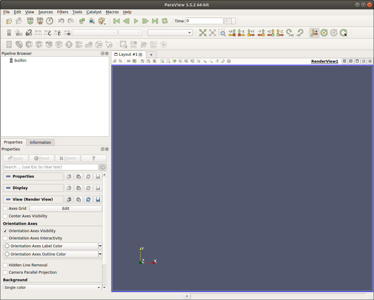{#figparaview width=“10cm”}

It is preferable to reproduce a high-resolution figure of particle configuration using post-processing softwares instead of a screenshot. As a demonstration, we load a state file named "shearend.xml.bz2" and output a vtk file or a pov file for post visualization.

1
2
3

O.load("shearend.xml.bz2")
import sudodem._superquadrics_utils as superutils
superutils.outputVTK("shearend.vtk",15)

Open Paraview, then import the vtk file "shearend.vtk" and click the button "Apply", so that the configuration of particles is visualized as shown in Fig. 4.2{reference-type=“ref” reference=“figshearendvtk”}. It is noteworthy that the function outputVTK processes a particle surface as a combination of many (determined by the argument slices, i.e., 15 herein) polygons, which would yield a large file (around 180 Mb in the presented example). The users may find ways to reduce the vtk file for a faster visualization in Paraview. One possible way is to show only the particles exposed in the view. Another possible way is to use the interface of built-in Superquadric source in Paraview.

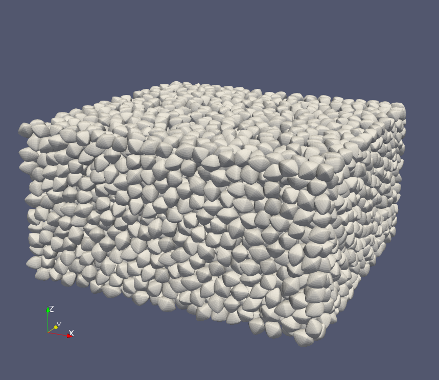{#figshearendvtk width=“8cm”}

Another alternative approach is rendering the scene utilizing POV-Ray.

1
2
3

O.load("shearend.xml.bz2")
import sudodem._superquadrics_utils as superutils
superutils.outputPOV("shearend.pov")

The users might revise the parameters of the camera in the POV file, i.e., "shearend.pov" here,

1
2
3
4
5
6
7

camera{ //orthographic angle 45
        location <0.6,0.6,0.5>*50e-3
        sky z
        look_at  <0,0,0.05>*10e-3
        right x*image_width/image_height
        translate <-0.04,0.01,-0.1>*50e-3
      }

Light sources should be slightly adjusted as well.

1
2
3
4
5

// White background
background{rgb 1}
// Two lights with slightly different colors
light_source{<4,8,5>*10e-3 color rgb <1,1,1>}
light_source{<12,-6>*10e-3 color rgb <1,1,1>}

In a terminal, run the following command to render the scene:

povray shearend.pov

For a high-resolution render, additional arguments are appended to the command,

povray shearend.pov +A0.01 +W1600 +H1200

Image processing softwares, e.g., GIMP [^8], can be used to change image size or make a gif animation, etc. Fig. 4.3{reference-type=“ref” reference=“figshearend”} shows configuration of particles rendered by POV-Ray and cropped using GIMP.

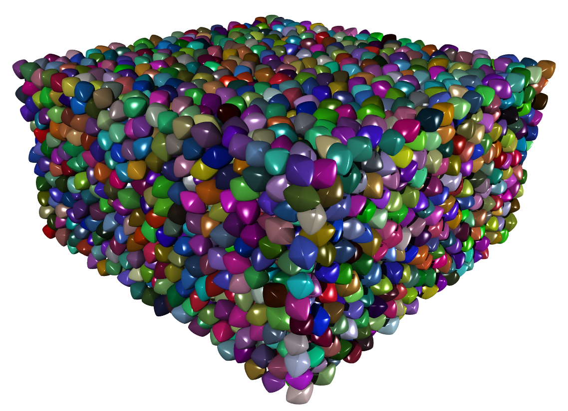{#figshearend width=“8cm”}

The module snapshot provides functions for visualizing poly-superellipsoids. As an example, we load the state of final packing, and import the module and call the outPov function as follows:

1
2

from sudodem import snapshot
snapshot.outPov("packingpolysuper",withbox=False)

we then get two files packingpolysuper.inc and packingpolysuper.pov. The first file packingpolysuper.inc includes macros for the definition of poly-superellipsoid and the particle information such as shape parameters, positions and orientations, like this:

 1
 2
 3
 4
 5
 6
 7
 8
 9
10
11
12
13
14
15
16
17
18
19
20
21
22
23
24
25
26
27
28
29
30
31
32
33
34
35

#macro myremain(sign1,sign2,sign3)
    clipped_by{plane{-sign1*x,0}}
    clipped_by{plane{-sign2*y,0}}
    clipped_by{plane{-sign3*z,0}}
#end
#macro randomColor(r,g,b)
texture{ pigment{ color rgb<r,g,b> transmit para_trans} finish { phong para_phong }}
#end
#macro octantSuper(ep1,ep2,rx,ry,rz,sign1,sign2,sign3)
    superellipsoid{ <ep1,ep2> 
#if (singleColor = false)
 randomColor(rand(Random_r),rand(Random_g),rand(Random_b)) 
#end
myremain(sign1,sign2,sign3) scale <rx,ry,rz>}
#end
#macro polySuperEllipsoid(ep1,ep2,a1,a2,b1,b2,c1,c2,t1,t2,t3,r1,r2,r3,r,g,b)
union{
octantSuper(ep1,ep2,a2,b2,c2,-1,-1,-1)
octantSuper(ep1,ep2,a1,b2,c2,1,-1,-1)
octantSuper(ep1,ep2,a2,b1,c2,-1,1,-1)
octantSuper(ep1,ep2,a1,b1,c2,1,1,-1)
octantSuper(ep1,ep2,a2,b2,c1,-1,-1,1)
octantSuper(ep1,ep2,a1,b2,c1,1,-1,1)
octantSuper(ep1,ep2,a2,b1,c1,-1,1,1)
octantSuper(ep1,ep2,a1,b1,c1,1,1,1)
rotate<r1,r2,r3>
translate<t1,t2,t3>
#if (singleColor = true)
randomColor(r,g,b)
#end
}
#end
polySuperEllipsoid(1.0000000e+00,1.0000000e+00,1.0000000e-01, 5.0000000e-02,8.0000000e-02,1.5000000e-01,2.0000000e-02, 4.0000000e-02,-3.2218276e-01,1.8390308e-01,3.1674861e-01, -167.727379,16.417442,-104.719219,0.783099,0.394383,0.840188)
...
...

The users are not suggested to edit this file though. But the second file packingpolysuper.pov includes some editable parameters as introduced above, and looks like this:

 1
 2
 3
 4
 5
 6
 7
 8
 9
10
11
12
13
14
15
16
17
18
19
20

//using the command: povray **.pov +A0.01 +W1600 +H1200
#include "colors.inc"
#declare singleColor =  true;
#declare Random_r = seed (1432);
#declare Random_g = seed (7242);
#declare Random_b = seed (9912);
#declare para_trans =  0 ;
#declare para_phong =  1.0 ;
camera {
location < 1.39244459003 , 0.950562440499 , 0.605226784362 >
sky z
right -x*image_width/image_height
look_at < 0.612872382451 , 0.349255160637 , 0.430021966053 >
}
#include "packingellipses.inc"
light_source{<4,8,5>*10 color rgb <1,1,1>}
light_source{<12,-6>*10 color rgb <1,1,1>}
light_source { <0, 2, 10> White }
background{rgb 1}
plane { z, -5 pigment { checker Green White }}//you may comment out this line to remove the plane

Then render it in a fresh terminal by typing

povray packingpolysuper.pov +A0.01 +W1600 +H1200

you will get a nice figure with higher quality as Fig. 4.4{reference-type=“ref” reference=“figpolypov”}.

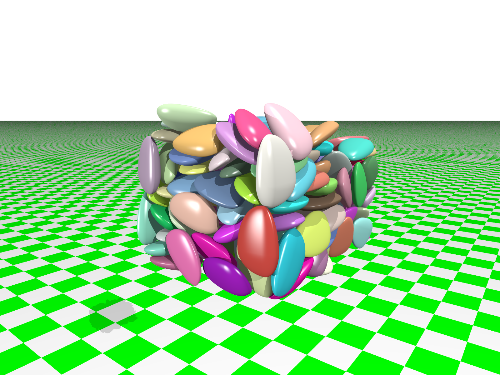{#figpolypov width=“10cm”}

SudoDEM2D

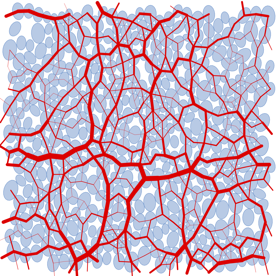
Module _superellipse_utils provides a function drawSVG (see Sec. 5.2.2{reference-type=“ref” reference=“secmodsuperellipse”}) to dump the particle profiles and contact forces chains to a SVG file.

1
2
3
4
5

from sudodem import _superellipse_utils
O.load("your data file")
drawSVG("test.svg", draw_forcechain=True,
                 force_line_color=(1.0,0,0),
                 solo_color=(93.0/255,152.0/255,208.0/255))

The output file test.svg is editable by using a text editor and/or Inkscape (recommended). Fig. 4.5{reference-type=“ref” reference=“figellipsesvg”} shows an exemplified snapshot of a packing of elliptic particles with periodic boundary conditions. Refer to the keywords of drawSVG for configuring the output figure.

{#figellipsesvg width=“10cm”}