后处理

如何后处理 SudoDEM 的模拟结果?

数据

用户可以使用PyRunner引擎来保存 SudoDEM 运行中的数据:

1
2
3
4
5
6
7
def savedata():
        global saving_num
        saving_num += 1
        #print "testing, no data saved"
        O.save('shear'+str(saving_num)+'.xml.bz2')  
        
O.engines = O.engines + [PyRunner( command = 'savedata()', iterPeriod = 1000 )] # if we load the consolidation data, then we do not need this line because the PyRunner calling 'savedata()' has been defined.

Python 包 utilspost 提供了一系列的后处理函数用来协助用户后处理,包括应力-力-组构计算以及用于调用其他后处理软件的接口函数 (例如,颗粒形状的vtk文件保存函数, 颗粒信息3D直方图的vtk文件保存函数)。基于如上包用户可以非常容易调用或自定义适合自己的后处理函数。

1
2
3
4
import sudodem.utilspost as utilspost
#如下函数可以帮助用户生成接触力发挥系数计算文件
for i in ['1.0','1.2','1.4','1.6']:
    utilspost.calc_avgFricMobilIndex(i,steps_num)

Python 包 _superquadrics_utils 提供如下后处理辅助函数,

  • outputParticles(filename) : 该函数接收一个文件名,并将保存每个颗粒的形状信息到该文件中,包括形状参数 $r_x$, $r_y$, $r_z$, $\epsilon_1$, $\epsilon_2$, 位置 $x$, $y$, $z$, 和朝向 $q0$,$q1$,$q2$,$q3$ (等价于 $q_w$, $q_x$, $q_y$, $q_z$)。

  • outputParticlesbyIds(filename, ids) : 该函数接收一个文件名以及颗粒索引,该函数将具有该索引的颗粒的信息保存到该文件中,保存信息与 outputParticles(filename) 相同。

  • outputWalls(filename) : 该函数接收一个文件名, 并将墙体的位置信息保存到该文件中。

  • outputPOV(filename) : 该函数接收一个文件名,并将颗粒的信息以POV-Ray文件格式保存,该POV-Ray文件可被用于POV-Ray进行颗粒的渲染。

  • outputVTK(filename,slices) : 该函数接收一个文件名,并将颗粒的信息以VTK文件格式保存,用户可以使用Paraview等VTK软件对颗粒进行渲染。

颗粒模拟可视化

SudoDEM3D

我们强烈推荐两款开源且免费的可视化软件用于 SudoDEM 的后处理可视化 Paraview[^6] and POV-Ray[^7]:

The main window of Paraview. {#figparaview width=“10cm”}

高精度的颗粒信息可视化相较于简单的截图可以更清晰表征模拟结果。这里我们将为大家演示如何利用vtk或者pov文件进行高精度颗粒信息可视化, 我们假设计算结果已经被保存至文件 "shearend.xml.bz2" 。

1
2
3
O.load("shearend.xml.bz2")
import sudodem._superquadrics_utils as superutils
superutils.outputVTK("shearend.vtk",15)

打开 Paraview, 导入vtk文件 "shearend.vtk" 然后点击按钮 "Apply" 从而得到如下图所示的可视化结果 Fig. 4.2{reference-type=“ref” reference=“figshearendvtk”}。 需要说明的是函数 outputVTK 将颗粒的表面视为多面体的切片组合 (切片的精度这里被设置为 15) , 依此法可能会得到较大的后处理文件 (该例子文件大约180 Mb)。 基于此用户可以选择多种多样的方式来减少后处理文件大小,比如用户可以通过 Paraview 提供的快速可视化方法,或者 可以利用 Paraview 内置接口 Superquadric 来降低可视化文件大小。

Configuration of particles rendered by
<em>Paraview</em>. 
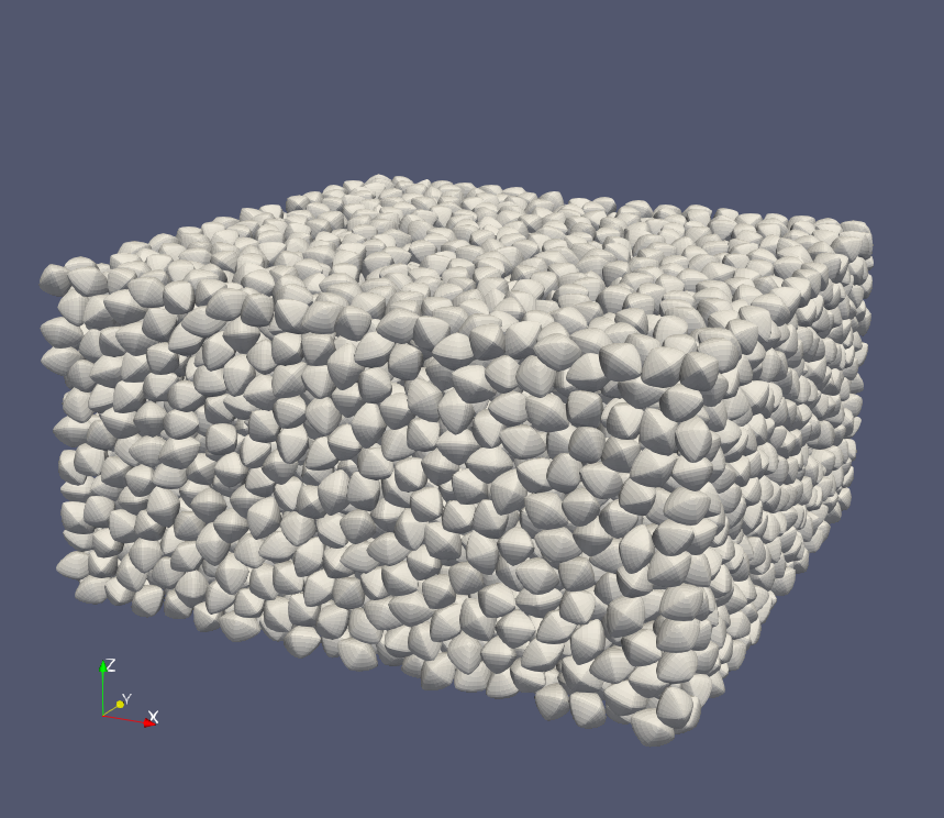
{#figshearendvtk width=“8cm”}

用户还可以通过使用POV-Ray 来降低可视化文件大小。

1
2
3
O.load("shearend.xml.bz2")
import sudodem._superquadrics_utils as superutils
superutils.outputPOV("shearend.pov")

用户可以通过修改POV文件的相机设置来达到自定义的可视化效果, i.e., "shearend.pov" here,

1
2
3
4
5
6
7
camera{ //orthographic angle 45
        location <0.6,0.6,0.5>*50e-3
        sky z
        look_at  <0,0,0.05>*10e-3
        right x*image_width/image_height
        translate <-0.04,0.01,-0.1>*50e-3
      }

这里给出了如何自定义光源的设置。

1
2
3
4
5
// White background
background{rgb 1}
// Two lights with slightly different colors
light_source{<4,8,5>*10e-3 color rgb <1,1,1>}
light_source{<12,-6>*10e-3 color rgb <1,1,1>}

在命令行中运行如下命令来可视化颗粒:

povray shearend.pov

如果要修改可视化精度,用户可以添加额外的命令参数来达到这一目的,

povray shearend.pov +A0.01 +W1600 +H1200

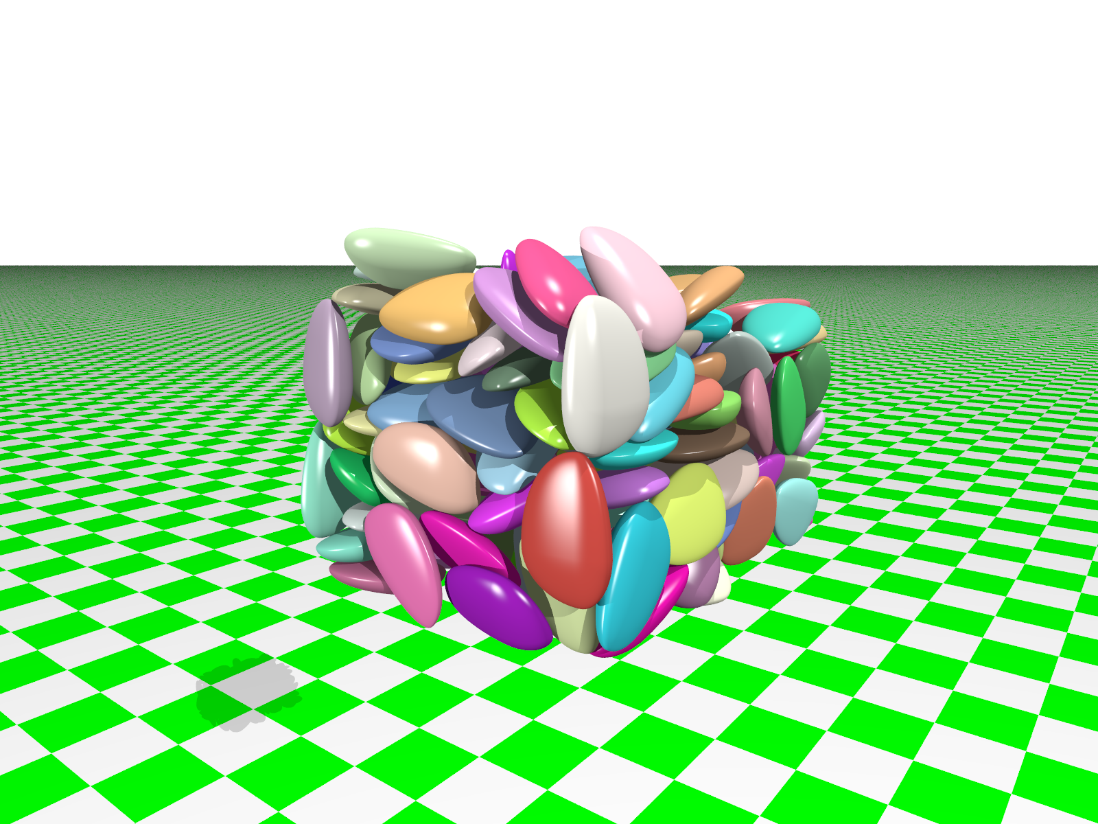
图像处理软件, 例如, GIMP [^8], 可用来修改图片大小或者制作动图。图 Fig. 4.3{reference-type=“ref” reference=“figshearend”} 给出了使用 POV-Ray 渲染并利用 GIMP 裁剪的颗粒渲染图片。

Configuration of particles rendered by
<em>POV-Ray</em>. {#figshearend width=“8cm”}

snapshot 提供了组合超椭球的可视化函数。例如,我们导入堆积结果完成时的颗粒状态文件并利用 snapshot 进行POV文件生成:

1
2
from sudodem import snapshot
snapshot.outPov("packingpolysuper",withbox=False)

此处我们得到两个文件分别是 packingpolysuper.incpackingpolysuper.pov。 第一个文件 packingpolysuper.inc 包含了一些组合超椭球的宏定义以及颗粒形状参数信息,例如颗粒形状参数,颗粒位置,颗粒朝向等

 1
 2
 3
 4
 5
 6
 7
 8
 9
10
11
12
13
14
15
16
17
18
19
20
21
22
23
24
25
26
27
28
29
30
31
32
33
34
35
#macro myremain(sign1,sign2,sign3)
    clipped_by{plane{-sign1*x,0}}
    clipped_by{plane{-sign2*y,0}}
    clipped_by{plane{-sign3*z,0}}
#end
#macro randomColor(r,g,b)
texture{ pigment{ color rgb<r,g,b> transmit para_trans} finish { phong para_phong }}
#end
#macro octantSuper(ep1,ep2,rx,ry,rz,sign1,sign2,sign3)
    superellipsoid{ <ep1,ep2> 
#if (singleColor = false)
 randomColor(rand(Random_r),rand(Random_g),rand(Random_b)) 
#end
myremain(sign1,sign2,sign3) scale <rx,ry,rz>}
#end
#macro polySuperEllipsoid(ep1,ep2,a1,a2,b1,b2,c1,c2,t1,t2,t3,r1,r2,r3,r,g,b)
union{
octantSuper(ep1,ep2,a2,b2,c2,-1,-1,-1)
octantSuper(ep1,ep2,a1,b2,c2,1,-1,-1)
octantSuper(ep1,ep2,a2,b1,c2,-1,1,-1)
octantSuper(ep1,ep2,a1,b1,c2,1,1,-1)
octantSuper(ep1,ep2,a2,b2,c1,-1,-1,1)
octantSuper(ep1,ep2,a1,b2,c1,1,-1,1)
octantSuper(ep1,ep2,a2,b1,c1,-1,1,1)
octantSuper(ep1,ep2,a1,b1,c1,1,1,1)
rotate<r1,r2,r3>
translate<t1,t2,t3>
#if (singleColor = true)
randomColor(r,g,b)
#end
}
#end
polySuperEllipsoid(1.0000000e+00,1.0000000e+00,1.0000000e-01, 5.0000000e-02,8.0000000e-02,1.5000000e-01,2.0000000e-02, 4.0000000e-02,-3.2218276e-01,1.8390308e-01,3.1674861e-01, -167.727379,16.417442,-104.719219,0.783099,0.394383,0.840188)
...
...

我们不建议用户直接修改第一个文件,但是用户可以通过修改第二个文件来达到自定义渲染效果:

 1
 2
 3
 4
 5
 6
 7
 8
 9
10
11
12
13
14
15
16
17
18
19
20
//using the command: povray **.pov +A0.01 +W1600 +H1200
#include "colors.inc"
#declare singleColor =  true;
#declare Random_r = seed (1432);
#declare Random_g = seed (7242);
#declare Random_b = seed (9912);
#declare para_trans =  0 ;
#declare para_phong =  1.0 ;
camera {
location < 1.39244459003 , 0.950562440499 , 0.605226784362 >
sky z
right -x*image_width/image_height
look_at < 0.612872382451 , 0.349255160637 , 0.430021966053 >
}
#include "packingellipses.inc"
light_source{<4,8,5>*10 color rgb <1,1,1>}
light_source{<12,-6>*10 color rgb <1,1,1>}
light_source { <0, 2, 10> White }
background{rgb 1}
plane { z, -5 pigment { checker Green White }}//you may comment out this line to remove the plane

命令行输入以下命令来完成渲染

povray packingpolysuper.pov +A0.01 +W1600 +H1200

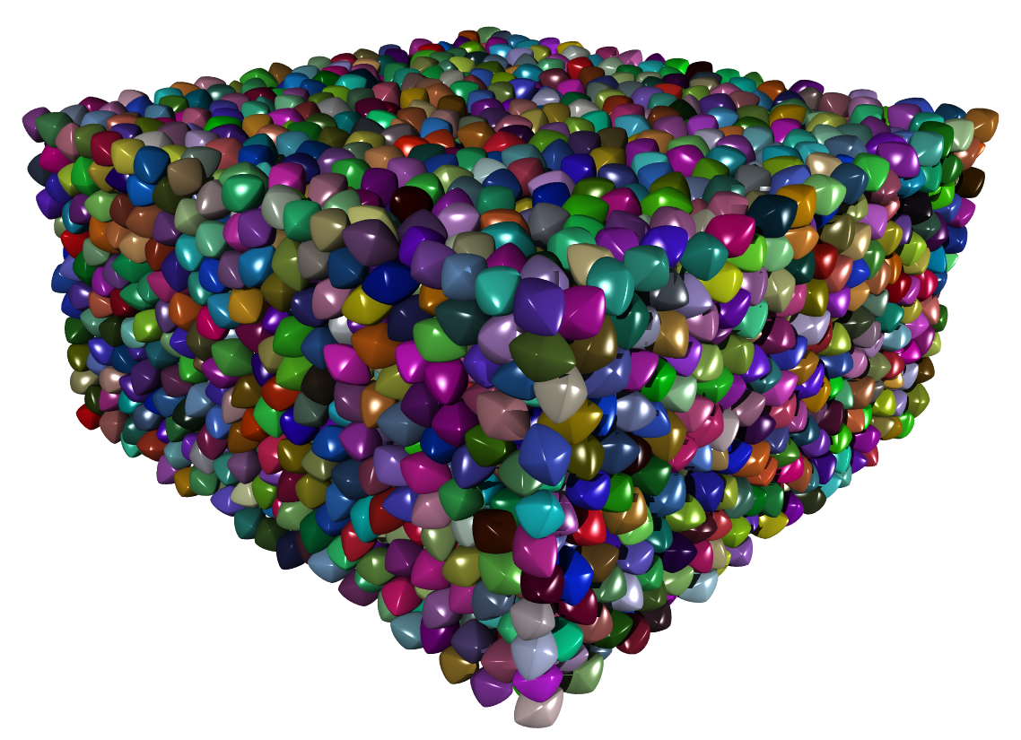
渲染完毕后用户将会得到如图所示的高精度后处理图片 Fig. 4.4{reference-type=“ref” reference=“figpolypov”}.

Packing of poly-superellipsoids in Example 4 rendered by
<em>POV-Ray</em>. {#figpolypov width=“10cm”}

SudoDEM2D

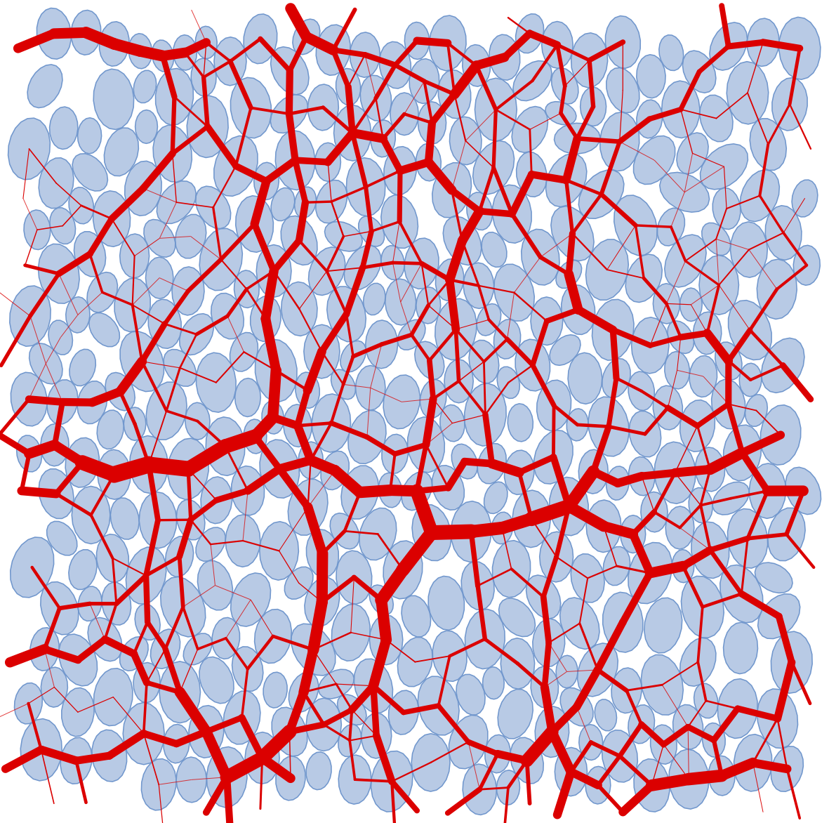
包 _superellipse_utils 提供了名为 drawSVG (see Sec. 5.2.2{reference-type=“ref” reference=“secmodsuperellipse”}) 的函数用于绘制颗粒力链的矢量图。

1
2
3
4
5
from sudodem import _superellipse_utils
O.load("your data file")
drawSVG("test.svg", draw_forcechain=True,
                 force_line_color=(1.0,0,0),
                 solo_color=(93.0/255,152.0/255,208.0/255))

生成的矢量图文件可以通过文本编辑器或者矢量图编辑器 Inkscape (推荐)来修改。图 Fig. 4.5{reference-type=“ref” reference=“figellipsesvg”} 给出了椭球颗粒在周期边界条件下堆积过程结束后的力链矢量图示例,用户可通过 drawSVG 函数来配置对应的输出图片格式。

Particles and contact force chains dumped by
<em>drawSVG</em>. {#figellipsesvg width=“10cm”}